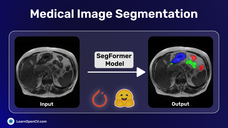
Medical image segmentation is an innovative process that enables surgeons to have a virtual “x-ray vision.” It is a highly valuable tool in healthcare, providing non-invasive diagnostics and in-depth analysis. With this in mind, in this post, we will explore the UW-Madison GI Tract Image Segmentation Kaggle challenge dataset. As part of this project, we will utilize PyTorch along with PyTorch-Lightning. We will use 🤗 HuggingFace transformers to load and fine-tune the Segformer transformer-based model on the medical segmentation dataset. Finally, we will create a Gradio app for image inference and deploy it on HuggingFace spaces.
- What is Medical Image Segmentation?
- What Are The Problems Faced In Medical Image Segmentation?
- Building The Medical Image Segmentation Dataset
- Install & Import Required Libraries
- Set Hyperparameters For The Project
- Loading The Medical Image Segmentation Dataset
- Using SegFormer Transformer Model From 🤗 HuggingFace
- Evaluation Metric & Loss Function
- Creating Custom LightningModule Class
- Start Training
- Inference on the Medical Segmentation Dataset
- Building The Gradio App
- Summary
Designed for those familiar with the basics of multi-head attention, PyTorch, and image segmentation, this blog post aims to enrich your knowledge of medical image segmentation. We will guide you through every step, from dataset creation and training to deploying an inference model. We’ve crafted our explanations to be accessible, ensuring learners at all levels can benefit.
What is Medical Image Segmentation?

Medical image segmentation is a process that involves dividing medical images, such as CT scans or MRI scans, into distinct regions or structures of interest. This technique is used to identify and isolate specific areas within the image, which is crucial for diagnosis, treatment planning, and monitoring of diseases. It can be done manually by experts or automated using computer algorithms and machine learning. Medical image segmentation plays a vital role in various medical specialties and enables quantitative analysis and precise measurements.
The dataset for this project is taken from the UW-Madison GI Tract Image Segmentation Kaggle competition. The dataset consists of 3 classes: the stomach, small bowel, and large bowel.

About the competition:
In 2019, an estimated 5 million people were diagnosed with a cancer of the gastro-intestinal tract worldwide. Of these patients, about half are eligible for radiation therapy, usually delivered over 10-15 minutes a day for 1-6 weeks. Radiation oncologists try to deliver high doses of radiation using X-ray beams pointed to tumors while avoiding the stomach and intestines. With newer technology such as integrated magnetic resonance imaging and linear accelerator systems, also known as MR-Linacs, oncologists are able to visualize the daily position of the tumor and intestines, which can vary day to day. In these scans, radiation oncologists must manually outline the position of the stomach and intestines in order to adjust the direction of the x-ray beams to increase the dose delivery to the tumor and avoid the stomach and intestines. This is a time-consuming and labor intensive process that can prolong treatments from 15 minutes a day to an hour a day, which can be difficult for patients to tolerate—unless deep learning could help automate the segmentation process. A method to segment the stomach and intestines would make treatments much faster and would allow more patients to get more effective treatment.
– Motivation behind the UW-Madison GI Tract Image Segmentation Kaggle competition
In this competition, the task was to develop a model that can automatically segment the stomach and intestines in MRI scans. These scans come from real cancer patients who underwent 1-5 MRI scans during radiation treatment on different days. By utilizing a dataset of these scans, you will leverage deep learning techniques to create innovative solutions that improve the quality of care for cancer patients.
What Are The Problems Faced In Medical Image Segmentation?
Medical image segmentation faces several challenges, including:
- Image variability: Diverse image characteristics make creating a universal segmentation algorithm challenging.
- Ambiguity and complexity: Complex structures, ambiguous boundaries, and overlapping regions complicate accurate segmentation.
- Limited labeled data: The scarcity of annotated medical images hampers developing and evaluating segmentation algorithms.
- Computational complexity: Large datasets and high-dimensional images require substantial computational resources and time.
- Validation and generalization: Ensuring accuracy and applicability across different modalities, populations, and clinical settings is difficult yet crucial.
Building The Medical Image Segmentation Dataset
As the task is to segment organ cells in images, the competition provides the dataset in the form of 16-bit grayscale PNG format images, and the ground-truth segmentation annotations are RLE-encoded masks provided in a CSV file.
Some 👀 observations about the dataset.
- It contains 115488 samples with multiple rows for each patient or case.
- Out of 115488 rows, only 33913 (29.364%) have RLE annotations for the class. This number denotes the total number of annotations available.
- The total number of images with corresponding annotations is 16590.
- These 16590 images belong to 85 cases/patients, where each patient has multiple scans for each day on multiple days.
- In these images:
- We have 8627 (~52%) annotations images for the Stomach.
- We have 11201 (~67.5%) annotations images for Small bowel.
- We have 14085 (~84.9%) annotations images for Large bowel.
- There are 2468 (~6.41%) samples with one annotation present.
- Of these, 2286 (~92.6%) are Stomach.
- Of these, 123 (~4.98%) are Large bowel.
- Of these, 59 (~2.39%) are Small bowel.
- There are 10921 (28.37%) samples with two annotations present.
- Of these, 7781 (~71.3%) are ‘Large bowel, Small bowel.’
- Of these, 2980 (~27.3%) are ‘Large bowel, Stomach.’
- Of these, 160 (~1.47%) are ‘Small bowel, Stomach.’
- Finally, 3,201 (8.32%) examples with all three classes are present.
UW-Madison GI Tract Medical Segmentation Dataset Preprocessing
Below is the entire Python script to preprocess the raw dataset to get the final one we used for the project.
The algorithm used is as follows:
- Traverse each “case” folder and record paths of all the images with annotations in the “train.csv” file using the
get_folder_files(...)function. - Split the image paths list in an 80:20 ratio for the training and validation set.
- Then we use the
create_and_write_img_msk(...)function to iterate over files of each set to:- Load and convert the image from uint16 to uint8 format using the
load_img(...)method. - Get the dataframe group (rows in “train.csv” file) for the image and decode the RLE-encoded mask for each class using
rle_decode(...)method for each image. Then the RGB mask is converted to a grayscale mask (single channel) where each pixel value indicates the class ID of the pixel. This process is done using thergb_to_onehot_to_gray(...)function. - Save image-mask pair in their respective folders.
- Load and convert the image from uint16 to uint8 format using the
Note:
- There are additional intermediate steps, such as extracting the folder name, sub-folder name, and image path of the image.
- The train.csv file contains image
ids in the format"case<num>_day<num>_slice_<slice_id>". Theget_folder_files(...)function, along with returning all the relevant image files in a “case” folder, returns a list ofimg_idswhich has the same format as the “train.csv”idcolumn. This is done to make it easier to fetch the relevant data frame rows during image and mask processing steps.
Script: all_in_one.py
# Import required libraries
import os
import re
import cv2
import numpy as np
import pandas as pd
from tqdm import tqdm
from sklearn.model_selection import train_test_split

"""
We've downloaded the "train" folder. The original train set images lie inside
the "original" folder.
"""
# Define paths for training dataset and image directory
TRAIN_CSV = "train.csv"
ORIG_IMG_DIR = os.path.join("original", "train")
CASE_FOLDERS = os.listdir(ORIG_IMG_DIR)

# Define paths for training and validation image and mask directories
ROOT_DATASET_DIR = "dataset_UWM_GI_Tract_train_valid"
ROOT_TRAIN_IMG_DIR = os.path.join(ROOT_DATASET_DIR, "train", "images")
ROOT_TRAIN_MSK_DIR = os.path.join(ROOT_DATASET_DIR, "train", "masks")
ROOT_VALID_IMG_DIR = os.path.join(ROOT_DATASET_DIR, "valid", "images")
ROOT_VALID_MSK_DIR = os.path.join(ROOT_DATASET_DIR, "valid", "masks")

# Create directories if not already present
os.makedirs(ROOT_TRAIN_IMG_DIR, exist_ok=True)
os.makedirs(ROOT_TRAIN_MSK_DIR, exist_ok=True)
os.makedirs(ROOT_VALID_IMG_DIR, exist_ok=True)
os.makedirs(ROOT_VALID_MSK_DIR, exist_ok=True)

# Define regular expressions to extract case, date, slice number, and image shape from file paths
GET_CASE_AND_DATE = re.compile(r"case[0-9]{1,3}_day[0-9]{1,3}")
GET_SLICE_NUM = re.compile(r"slice_[0-9]{1,4}")
IMG_SHAPE = re.compile(r"_[0-9]{1,3}_[0-9]{1,3}_")

# Load the main dataframe from csv file and drop rows with null values
MAIN_DF = pd.read_csv(TRAIN_CSV).dropna(axis=0)
only_IDS = MAIN_DF["id"].to_numpy()

# Define classes for image segmentation
CLASSES = ["large_bowel", "small_bowel", "stomach"]

# Create a mapping of class ID to RGB value
color2id = {
    (0, 0, 0): 0,  # background pixel
    (0, 0, 255): 1,  # Blue - Stomach
    (0, 255, 0): 2,  # Green - Small bowel
    (255, 0, 0): 3,  # Red - Large bowel
}

# Reverse map from id to color
id2color = {v: k for k, v in color2id.items()}


# Function to get all relevant image files in a given directory
def get_folder_files(folder_path):
    all_relevant_imgs_in_case = []
    img_ids = []

    for dir, _, files in os.walk(folder_path):
        if not len(files):
            continue

        for file_name in files:
            src_file_path = os.path.join(dir, file_name)

            case_day = GET_CASE_AND_DATE.search(src_file_path).group()
            slice_id = GET_SLICE_NUM.search(src_file_path).group()
            image_id = case_day + "_" + slice_id

            if image_id in only_IDS:
                all_relevant_imgs_in_case.append(src_file_path)
                img_ids.append(image_id)

    return all_relevant_imgs_in_case, img_ids


# Function to decode Run-Length Encoding (RLE) into an image mask
# ref: https://www.kaggle.com/paulorzp/run-length-encode-and-decode
def rle_decode(mask_rle, shape):
    """
    mask_rle: run-length as string formated (start length)
    shape: (height,width) of array to return
    Returns numpy array, 1 - mask, 0 - background

    """
    s = np.asarray(mask_rle.split(), dtype=int)
    starts = s[0::2] - 1
    lengths = s[1::2]
    ends = starts + lengths
    img = np.zeros(shape[0] * shape[1], dtype=np.uint8)
    for lo, hi in zip(starts, ends):
        img[lo:hi] = 1
    return img.reshape(shape)  # Needed to align to RLE direction


# Function to load and convert image from a uint16 to uint8 datatype.
def load_img(img_path):
    img = cv2.imread(img_path, cv2.IMREAD_UNCHANGED).astype(np.float32)
    img = (img - img.min()) / (img.max() - img.min()) * 255.0
    img = img.astype(np.uint8)
    img = np.tile(img[..., None], [1, 1, 3])  # gray to rgb
    return img


# Function to convert RGB image to one-hot encoded grayscale image based on color map.
def rgb_to_onehot_to_gray(rgb_arr, color_map=id2color):
    num_classes = len(color_map)
    shape = rgb_arr.shape[:2] + (num_classes,)
    arr = np.zeros(shape, dtype=np.float32)

    for i, cls in enumerate(color_map):
        arr[:, :, i] = np.all(rgb_arr.reshape((-1, 3)) == color_map[i], axis=1).reshape(shape[:2])

    return arr.argmax(-1)


# Function to create and write image-mask pair for each file path in given directories.
def create_and_write_img_msk(file_paths, file_ids, save_img_dir, save_msk_dir, desc=None):
    for file_path, file_id in tqdm(zip(file_paths, file_ids), ascii=True, total=len(file_ids), desc=desc, leave=True):
        image = load_img(file_path)

        IMG_DF = MAIN_DF[MAIN_DF["id"] == file_id]

        img_shape_H_W = list(map(int, IMG_SHAPE.search(file_path).group()[1:-1].split("_")))[::-1]
        mask_image = np.zeros(img_shape_H_W + [len(CLASSES)], dtype=np.uint8)

        for i, class_label in enumerate(CLASSES):
            class_row = IMG_DF[IMG_DF["class"] == class_label]

            if len(class_row):
                rle = class_row.segmentation.squeeze()
                mask_image[..., i] = rle_decode(rle, img_shape_H_W) * 255

        mask_image = rgb_to_onehot_to_gray(mask_image, color_map=id2color)

        FILE_CASE_AND_DATE = GET_CASE_AND_DATE.search(file_path).group()
        FILE_NAME = os.path.split(file_path)[-1]

        new_name = FILE_CASE_AND_DATE + "_" + FILE_NAME

        dst_img_path = os.path.join(save_img_dir, new_name)
        dst_msk_path = os.path.join(save_msk_dir, new_name)

        cv2.imwrite(dst_img_path, image)
        cv2.imwrite(dst_msk_path, mask_image)

    return


if __name__ == "__main__":
    # Set random seed for reproducibility
    np.random.seed(42)

    # Main script execution: for each folder, split the data into training and validation sets, and create/write image-mask pairs.
    for folder in CASE_FOLDERS:
        all_relevant_imgs_in_case, img_ids = get_folder_files(folder_path=os.path.join(ORIG_IMG_DIR, folder))
        train_files, valid_files, train_img_ids, valid_img_ids = train_test_split(all_relevant_imgs_in_case, img_ids, train_size=0.8, shuffle=True)
        create_and_write_img_msk(train_files, train_img_ids, ROOT_TRAIN_IMG_DIR, ROOT_TRAIN_MSK_DIR, desc=f"Train :: {folder}")
        create_and_write_img_msk(valid_files, valid_img_ids, ROOT_VALID_IMG_DIR, ROOT_VALID_MSK_DIR, desc=f"Valid :: {folder}")
        print()
Beginning from the next section, we’ll focus on the code implementation of the project. We’ll add all the explanations required to understand the procedures.
Install & Import Required Libraries
Before we begin the coding part, we must ensure all the required libraries are installed. For this project, apart from PyTorch, we are installing additional tools to help ease the implementation process.

The major ones are:
transformers: To load the SegFormer transformer model.lightning: To simplify and structure code implementations.torchmetrics: For evaluating the model’s performance.wandb: For experiment tracking.albumentations: For applying augmentations.
# Install libraries and restart kernel.
%pip install -qqqU wandb transformers lightning albumentations torchmetrics torchinfo
%pip install -qqq requests gradio
Let’s start
import os
import zipfile
import platform
import warnings
from glob import glob
from dataclasses import dataclass

# To filter UserWarning.
warnings.filterwarnings("ignore", category=UserWarning)

import cv2
import requests
import numpy as np
# from tqdm import tqdm
import matplotlib.pyplot as plt

import torch
import torch.nn as nn
import torch.optim as optim
import torch.nn.functional as F
from torch.utils.data import Dataset, DataLoader


# For data augmentation and preprocessing.
import albumentations as A
from albumentations.pytorch import ToTensorV2

# Imports required SegFormer classes
from transformers import SegformerForSemanticSegmentation

# Importing lighting along with a built-in callback it provides.
import lightning.pytorch as pl
from lightning.pytorch.loggers import WandbLogger
from lightning.pytorch.callbacks import LearningRateMonitor, ModelCheckpoint

# Importing torchmetrics modular and functional implementations.
from torchmetrics import MeanMetric
from torchmetrics.classification import MulticlassF1Score

# To print model summary.
from torchinfo import summary

# Sets the internal precision of float32 matrix multiplications.
torch.set_float32_matmul_precision('high')

# To enable determinism.
os.environ["CUBLAS_WORKSPACE_CONFIG"] = ":16:8"

# To render the matplotlib figure in the notebook.
%matplotlib inline
For this project, instead of the default tensorboard used by pytorch-lightning for tracking experiments, we will use a proper MLOps tool: Weights & Biases (WandB).
The following code cell will help us to log into our wandb account.
import wandb

wandb.login()
The code cell will ask you to paste your API key in the dialogue box. You need to click on the Sign In with Auth0 link provided.
Set Hyperparameters For The Project
Next, we will declare all the different hyperparameters used for the project. For this, we are defining three dataclasses. They will be used throughout the notebook.
- DatasetConfig – A class that holds all the hyperparameters we will use to process images. It contains the following information:
- Image size to use.
- Number of classes present in the dataset,
- The mean and standard deviation to use for image normalization.
- URL of the preprocessed dataset.
- Directory path to download the dataset to.
- Paths – This class contains the locations of the images and masks of the train and validation sets. It uses the “root dataset path” set DatasetConfig as the base.
- TrainingConfig – A class that holds all the hyperparameters we will use for training and evaluation. It contains the following information:
- Batch size.
- Initial learning rate.
- The number of epochs to train the model.
- The number of workers to use for data loading.
- Model, optimizer & learning rate scheduler-related configurations.
- InferenceConfig – This class contains the (optional) batch size and the number of batches we will use to display our inference results at the end.
Note: We’ve uploaded the preprocessed dataset to our Dropbox and Kaggle accounts. There are two options. You can manually download the dataset and move it to your workstation or utilize the data download code we’ve written below to do it automatically.
@dataclass(frozen=True)
class DatasetConfig:
    NUM_CLASSES:   int = 4 # including background.
    IMAGE_SIZE: tuple[int,int] = (288, 288) # W, H
    MEAN: tuple = (0.485, 0.456, 0.406)
    STD:  tuple = (0.229, 0.224, 0.225)
    BACKGROUND_CLS_ID: int = 0
    URL: str = r"https://www.dropbox.com/scl/fi/r0685arupp33sy31qhros/dataset_UWM_GI_Tract_train_valid.zip?rlkey=w4ga9ysfiuz8vqbbywk0rdnjw&dl=1"
    DATASET_PATH: str = os.path.join(os.getcwd(), "dataset_UWM_GI_Tract_train_valid")

@dataclass(frozen=True)
class Paths:
    DATA_TRAIN_IMAGES: str = os.path.join(DatasetConfig.DATASET_PATH, "train", "images", r"*.png")
    DATA_TRAIN_LABELS: str = os.path.join(DatasetConfig.DATASET_PATH, "train", "masks",  r"*.png")
    DATA_VALID_IMAGES: str = os.path.join(DatasetConfig.DATASET_PATH, "valid", "images", r"*.png")
    DATA_VALID_LABELS: str = os.path.join(DatasetConfig.DATASET_PATH, "valid", "masks",  r"*.png")

@dataclass
class TrainingConfig:
    BATCH_SIZE:      int = 48 # 32. On colab you should be able to use batch size of 32 with T4 GPU.
    NUM_EPOCHS:      int = 100
    INIT_LR:       float = 3e-4
    NUM_WORKERS:     int = 0 if platform.system() == "Windows" else 12 # os.cpu_count()

    OPTIMIZER_NAME:  str = "AdamW"
    WEIGHT_DECAY:  float = 1e-4
    USE_SCHEDULER:  bool = True # Use learning rate scheduler?
    SCHEDULER:       str = "MultiStepLR" # Name of the scheduler to use.
    MODEL_NAME:      str = "nvidia/segformer-b4-finetuned-ade-512-512"


@dataclass
class InferenceConfig:
    BATCH_SIZE:  int = 10
    NUM_BATCHES: int = 2
Loading The Medical Image Segmentation Dataset
As mentioned before, we use the pytorch-lightning library to remove the boilerplate code necessary when writing pure PyTorch code. To do so, we must ensure we follow the format as Lightning requires. To that end, we will create our custom class MedicalSegmentationDataModule that inherits from LightningDataModule.
Before we begin, we will declare a dictionary to map each class ID to their respective RGB color values.
# Create a mapping from class ID to RGB color value. Required for visualization.
id2color = {
    0: (0, 0, 0),    # background pixel
    1: (0, 0, 255),  # Stomach
    2: (0, 255, 0),  # Small Bowel
    3: (255, 0, 0),  # large Bowel
}

print("Number of classes", DatasetConfig.NUM_CLASSES)

# Reverse id2color mapping.
# Used for converting RGB mask to a single channel (grayscale) representation.
rev_id2color = {value: key for key, value in id2color.items()}
A Custom PyTorch Dataset Class For Medical Image Segmentation
First, we will define our custom PyTorch Dataset class. This custom is designed to load images and masks for each image. The Dataset class is essential for efficient and organized data handling in machine learning tasks. It provides a standardized interface to load and preprocess data samples from various sources. Encapsulating the dataset into a single object simplifies data management. It enables seamless integration with other PyTorch components like data loaders and models.
The custom class performs the following functions:
- Load each image-mask pair.
- Apply geometric and pixel augmentations if the pair belongs to the training set.
- Apply preprocessing transformations such as normalization and standardization.
class MedicalDataset(Dataset):
    def __init__(self, *, image_paths, mask_paths, img_size, ds_mean, ds_std, is_train=False):
        self.image_paths = image_paths
        self.mask_paths  = mask_paths
        self.is_train    = is_train
        self.img_size    = img_size
        self.ds_mean = ds_mean
        self.ds_std = ds_std
        self.transforms  = self.setup_transforms(mean=self.ds_mean, std=self.ds_std)

    def __len__(self):
        return len(self.image_paths)

    def setup_transforms(self, *, mean, std):
        transforms = []

        # Augmentation to be applied to the training set.
        if self.is_train:
            transforms.extend([
                A.HorizontalFlip(p=0.5), A.VerticalFlip(p=0.5),
                A.ShiftScaleRotate(scale_limit=0.12, rotate_limit=0.15, shift_limit=0.12, p=0.5),
                A.RandomBrightnessContrast(p=0.5),
                A.CoarseDropout(max_holes=8, max_height=self.img_size[1]//20, max_width=self.img_size[0]//20, min_holes=5, fill_value=0, mask_fill_value=0, p=0.5)
            ])

        # Preprocess transforms - Normalization and converting to PyTorch tensor format (HWC --> CHW).
        transforms.extend([
                A.Normalize(mean=mean, std=std, always_apply=True),
                ToTensorV2(always_apply=True),  # (H, W, C) --> (C, H, W)
        ])
        return A.Compose(transforms)

    def load_file(self, file_path, depth=0):
        file = cv2.imread(file_path, depth)
        if depth == cv2.IMREAD_COLOR:
            file = file[:, :, ::-1]
        return cv2.resize(file, (self.img_size), interpolation=cv2.INTER_NEAREST)

    def __getitem__(self, index):
        # Load image and mask file.
        image = self.load_file(self.image_paths[index], depth=cv2.IMREAD_COLOR)
        mask  = self.load_file(self.mask_paths[index],  depth=cv2.IMREAD_GRAYSCALE)

        # Apply Preprocessing (+ Augmentations) transformations to image-mask pair
        transformed = self.transforms(image=image, mask=mask)
        image, mask = transformed["image"], transformed["mask"].to(torch.long)
        return image, mask
Defining The Custom LightningDataModule Class
In this section, we will define the custom MedicalSegmentationDataModule class inherited from Lightning’s LightningDataModule class. It helps organize and encapsulate all the data-related operations and logic in a PyTorch project. It acts as a bridge between your data and Lightning’s training pipeline. It is a convenient abstraction that encapsulates data-related operations, promotes code organization, and facilitates seamless integration with other Lightning components for efficient and reproducible deep-learning experiments.
The class will perform the following functions:
- Download the dataset from Dropbox.
- Create a
MedicalDatasetclass object for each set. - Create and return the
DataLoaderobjects for each set.
The class methods we need to define are as follows:
prepare_data(..): This method is used for data preparation, like downloading and one-time preprocessing with the dataset. When training in a distributed setting, this will be called from each GPU machine.setup(...): When you want to perform data operations on every GPU, this method is apt for it will call from every GPU. For example, perform train/val/test splits.train_dataloader(...): This method returns the train dataloader.val_dataloader(...): This method returns validation dataloader.
class MedicalSegmentationDataModule(pl.LightningDataModule):
    def __init__(
        self,
        num_classes=10,
        img_size=(384, 384),
        ds_mean=(0.485, 0.456, 0.406),
        ds_std=(0.229, 0.224, 0.225),
        batch_size=32,
        num_workers=0,
        pin_memory=False,
        shuffle_validation=False,
    ):
        super().__init__()

        self.num_classes = num_classes
        self.img_size    = img_size
        self.ds_mean     = ds_mean
        self.ds_std      = ds_std
        self.batch_size  = batch_size
        self.num_workers = num_workers
        self.pin_memory  = pin_memory

        self.shuffle_validation = shuffle_validation

    def prepare_data(self):
        # Download dataset.
        dataset_zip_path = f"{DatasetConfig.DATASET_PATH}.zip"

        # Download if dataset does not exists.
        if not os.path.exists(DatasetConfig.DATASET_PATH):

            print("Downloading and extracting assets...", end="")
            file = requests.get(DatasetConfig.URL)
            open(dataset_zip_path, "wb").write(file.content)

            try:
                with zipfile.ZipFile(dataset_zip_path) as z:
                    z.extractall(os.path.split(dataset_zip_path)[0]) # Unzip where downloaded.
                    print("Done")
            except:
                print("Invalid file")

            os.remove(dataset_zip_path) # Remove the ZIP file to free storage space.

    def setup(self, *args, **kwargs):
        # Create training dataset and dataloader.
        train_imgs = sorted(glob(f"{Paths.DATA_TRAIN_IMAGES}"))
        train_msks  = sorted(glob(f"{Paths.DATA_TRAIN_LABELS}"))

        # Create validation dataset and dataloader.
        valid_imgs = sorted(glob(f"{Paths.DATA_VALID_IMAGES}"))
        valid_msks = sorted(glob(f"{Paths.DATA_VALID_LABELS}"))

        self.train_ds = MedicalDataset(image_paths=train_imgs, mask_paths=train_msks, img_size=self.img_size,
                                       is_train=True, ds_mean=self.ds_mean, ds_std=self.ds_std)

        self.valid_ds = MedicalDataset(image_paths=valid_imgs, mask_paths=valid_msks, img_size=self.img_size,
                                       is_train=False, ds_mean=self.ds_mean, ds_std=self.ds_std)

    def train_dataloader(self):
        # Create train dataloader object with drop_last flag set to True.
        return DataLoader(
            self.train_ds, batch_size=self.batch_size,  pin_memory=self.pin_memory,
            num_workers=self.num_workers, drop_last=True, shuffle=True
        )

    def val_dataloader(self):
        # Create validation dataloader object.
        return DataLoader(
            self.valid_ds, batch_size=self.batch_size,  pin_memory=self.pin_memory,
            num_workers=self.num_workers, shuffle=self.shuffle_validation
        )
Usage: Let’s download the dataset and initialize train and validation data loaders. We’ll use them to visualize the dataset.
%%time

dm = MedicalSegmentationDataModule(
    num_classes=DatasetConfig.NUM_CLASSES,
    img_size=DatasetConfig.IMAGE_SIZE,
    ds_mean=DatasetConfig.MEAN,
    ds_std=DatasetConfig.STD,
    batch_size=InferenceConfig.BATCH_SIZE,
    num_workers=0,
    shuffle_validation=True,
)

# Donwload dataset.
dm.prepare_data()

# Create training & validation dataset.
dm.setup()

train_loader, valid_loader = dm.train_dataloader(), dm.val_dataloader()
Some Helper Function To Visualize the Medical Segmentation Dataset
To help visualize our dataset, we need to define some additional helper functions. They are as follows:
A) num_to_rgb(...): Function will be used to convert single-channel mask representations to an integrated RGB mask for visualization purposes.
def num_to_rgb(num_arr, color_map=id2color):
    single_layer = np.squeeze(num_arr)
    output = np.zeros(num_arr.shape[:2] + (3,))

    for k in color_map.keys():
        output[single_layer == k] = color_map[k]

    # return a floating point array in range [0.0, 1.0]
    return np.float32(output) / 255.0
B) image_overlay(...): This function overlays an RGB segmentation map on top of an RGB image.
def image_overlay(image, segmented_image):
    alpha = 1.0  # Transparency for the original image.
    beta = 0.7  # Transparency for the segmentation map.
    gamma = 0.0  # Scalar added to each sum.

    segmented_image = cv2.cvtColor(segmented_image, cv2.COLOR_RGB2BGR)

    image = cv2.cvtColor(image, cv2.COLOR_RGB2BGR)

    image = cv2.addWeighted(image, alpha, segmented_image, beta, gamma, image)
    image = cv2.cvtColor(image, cv2.COLOR_BGR2RGB)

    return np.clip(image, 0.0, 1.0)
C) display_image_and_mask(...): The convenience function below will display the original image, the ground truth mask, and the ground truth mask overlayed on the original image.
def display_image_and_mask(*, images, masks, color_map=id2color):
    title = ["GT Image", "Color Mask", "Overlayed Mask"]

    for idx in range(images.shape[0]):
        image = images[idx]
        grayscale_gt_mask = masks[idx]

        fig = plt.figure(figsize=(15, 4))

        # Create RGB segmentation map from grayscale segmentation map.
        rgb_gt_mask = num_to_rgb(grayscale_gt_mask, color_map=color_map)

        # Create the overlayed image.
        overlayed_image = image_overlay(image, rgb_gt_mask)

        plt.subplot(1, 3, 1)
        plt.title(title[0])
        plt.imshow(image)
        plt.axis("off")

        plt.subplot(1, 3, 2)
        plt.title(title[1])
        plt.imshow(rgb_gt_mask)
        plt.axis("off")

        plt.imshow(rgb_gt_mask)
        plt.subplot(1, 3, 3)
        plt.title(title[2])
        plt.imshow(overlayed_image)
        plt.axis("off")

        plt.tight_layout()
        plt.show()

    return
D) denormalize(...): This function is used to denormalize the image tensors and clip values between 0 and 1. It is used to denormalize the images for visualization.
def denormalize(tensors, *, mean, std):
    for c in range(DatasetConfig.CHANNELS):
        tensors[:, c, :, :].mul_(std[c]).add_(mean[c])

    return torch.clamp(tensors, min=0.0, max=1.0)
Display Sample Images From The Validation Dataset
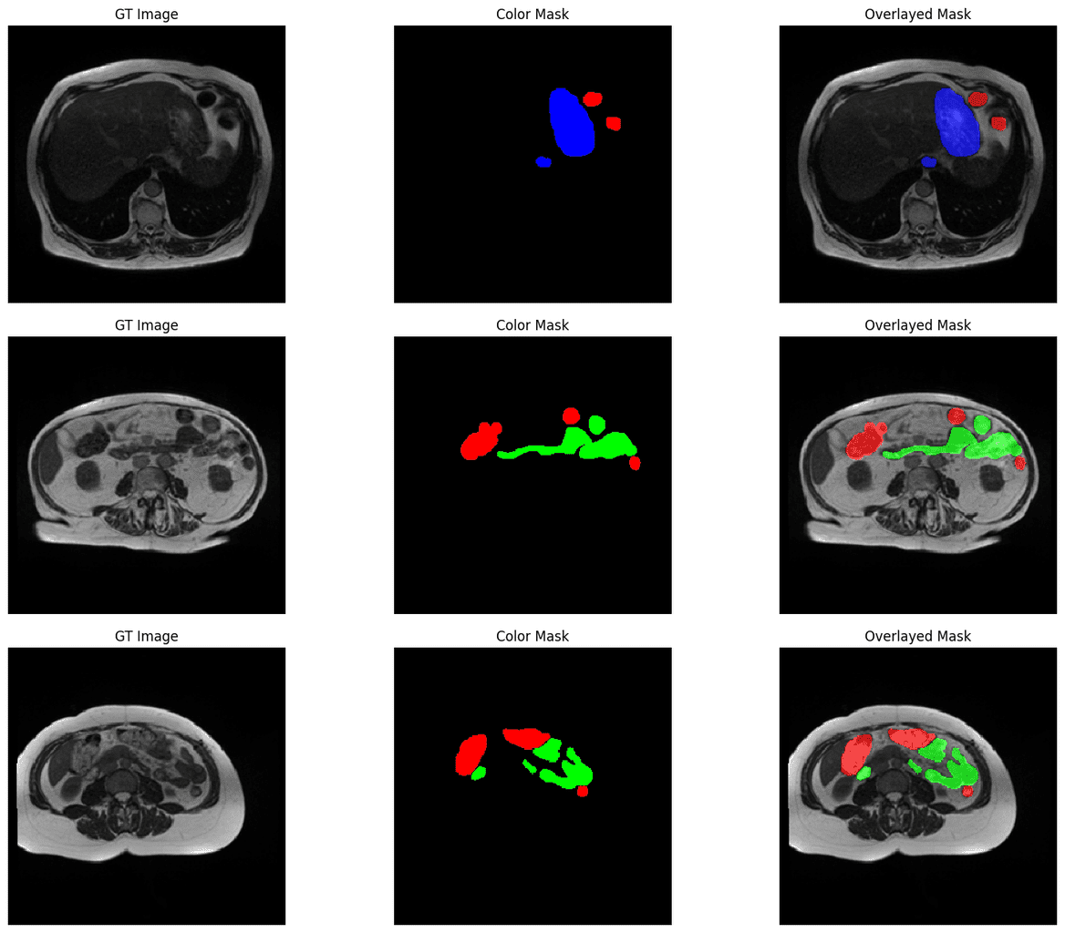
We will loop over the first batch in the validation dataset and display the ground truth image, ground truth mask, and the ground truth mask overlayed on the image. The overlay helps us to better understand the segmented classes in the context of the original image.
for batch_images, batch_masks in valid_loader:

    batch_images = denormalize(batch_images, mean=DatasetConfig.MEAN, std=DatasetConfig.STD).permute(0, 2, 3, 1).numpy()
    batch_masks  = batch_masks.numpy()

    print("batch_images shape:", batch_images.shape)
    print("batch_masks shape: ", batch_masks.shape)

    display_image_and_mask(images=batch_images, masks=batch_masks)

    break
Here are some samples:
Using SegFormer Transformer Model From 🤗 HuggingFace
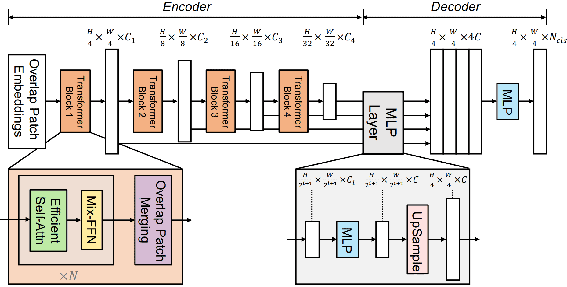
The SegFormer model was proposed in the paper titled SegFormer: Simple and Efficient Design for Semantic Segmentation with Transformers. The model consists of a hierarchical Transformer encoder made of efficient multi-head attention modules and a final lightweight all-MLP decoder head.
Paper abstract
“We present SegFormer, a simple, efficient yet powerful semantic segmentation framework which unifies Transformers with lightweight multilayer perception (MLP) decoders. SegFormer has two appealing features: 1) SegFormer comprises a novel hierarchically structured Transformer encoder which outputs multiscale features. It does not need positional encoding, thereby avoiding the interpolation of positional codes which leads to decreased performance when the testing resolution differs from training. 2) SegFormer avoids complex decoders. The proposed MLP decoder aggregates information from different layers, and thus combining both local attention and global attention to render powerful representations. We show that this simple and lightweight design is the key to efficient segmentation on Transformers. We scale our approach up to obtain a series of models from SegFormer-B0 to SegFormer-B5, reaching significantly better performance and efficiency than previous counterparts. For example, SegFormer-B4 achieves 50.3% mIoU on ADE20K with 64M parameters, being 5x smaller and 2.2% better than the previous best method. Our best model, SegFormer-B5, achieves 84.0% mIoU on Cityscapes validation set and shows excellent zero-shot robustness on Cityscapes-C.”
– SegFormer: Simple and Efficient Design for Semantic Segmentation with Transformers
You can check all the trained weights available for the SegFormer model on HuggingFace.
Loading a pre-trained model version and getting it ready for inference or finetuning is very easy, thanks to HuggingFace.
We only have to pass the following:
pretrained_model_name_or_path: (string) The id/path of a pre-trained model hosted on the Huggingface model zoo.num_labels: (int) The number of channels (one for each class) we want the model to give as output. Suppose the number differs from the original number. In that case, the layer will be replaced with a new layer with randomly initialized weights.ignore_mismatched_sizes: (bool) Boolean value to whether or not to ignore the weight key mismatch. Here, it occurs because we change the num_labels value.
Function definition:
def get_model(*, model_name, num_classes):
    model = SegformerForSemanticSegmentation.from_pretrained(
        model_name,
        num_labels=num_classes,
        ignore_mismatched_sizes=True,
    )
    return model
Usage
model = get_model(model_name=TrainingConfig.MODEL_NAME, num_classes=DatasetConfig.NUM_CLASSES)
- The model’s forward pass takes multiple arguments [Segformer documentation]. The two important ones are
pixel_valuesandlabels. - The
pixel_valuesargument refers to the input images. Thelabelsargument is for passing the ground-truth mask. - If
labelsare passed, the model’s forward pass calculates the cross-entropy (CE) loss. - The output logits are smaller than the input image size. To get the outputs to match the input image size, we need to upsample it simply.
Create dummy inputs.
data    = torch.randn(1, 3, *DatasetConfig.IMAGE_SIZE[::-1])
target = torch.rand(1, *DatasetConfig.IMAGE_SIZE[::-1]).to(torch.long)
Generate dummy outputs.
outputs = model(pixel_values=data, labels=target, return_dict=True)

# Upsample model outputs to match input image size.
upsampled_logits = F.interpolate(outputs["logits"], size=target.shape[-2:], mode="bilinear", align_corners=False)
To access the model’s output, we have to use the "logits" key. Similarly, we can access the loss via the "loss" key.
print("Model Outputs: outputs['logits']:", outputs["logits"].shape)
print("Model Outputs Resized::", upsampled_logits.shape)
print("Loss: outputs['loss']:", outputs["loss"])
Outputs:

Model Outputs: outputs['logits']: torch.Size([1, 4, 72, 72])
Model Outputs Resized:: torch.Size([1, 4, 288, 288])
Loss: outputs['loss']: tensor(1.3995, grad_fn=<NllLoss2DBackward0>)
In this project, we won’t be using the CE loss returned by the model for training. Instead, we will define our custom combo loss function that combines the Smooth Dice coefficient & CE to compute the loss.
Print model summary:
summary(model, input_size=(1, 3, *DatasetConfig.IMAGE_SIZE[::-1]), depth=2, device="cpu")
=============================================================================================================================
Layer (type:depth-idx)                                                      Output Shape              Param #
=============================================================================================================================
SegformerForSemanticSegmentation                                            [1, 4, 72, 72]            --
├─SegformerModel: 1-1                                                       [1, 64, 72, 72]           --
│    └─SegformerEncoder: 2-1                                                [1, 64, 72, 72]           60,842,688
├─SegformerDecodeHead: 1-2                                                  [1, 4, 72, 72]            --
│    └─ModuleList: 2-2                                                      --                        789,504
│    └─Conv2d: 2-3                                                          [1, 768, 72, 72]          2,359,296
│    └─BatchNorm2d: 2-4                                                     [1, 768, 72, 72]          1,536
│    └─ReLU: 2-5                                                            [1, 768, 72, 72]          --
│    └─Dropout: 2-6                                                         [1, 768, 72, 72]          --
│    └─Conv2d: 2-7                                                          [1, 4, 72, 72]            3,076
=============================================================================================================================
Total params: 63,996,100
Trainable params: 63,996,100
Non-trainable params: 0
Total mult-adds (G): 14.02
=============================================================================================================================
Input size (MB): 1.00
Forward/backward pass size (MB): 694.74
Params size (MB): 255.98
Estimated Total Size (MB): 951.72
=============================================================================================================================
Evaluation Metric & Loss Function
The Dice Coefficient (otherwise known as the F1-Score) is a function commonly used in the context of segmentation and is often specifically used as the basis for a loss function for segmentation problems. We will write the custom loss function next based on the Dice Coefficient, but let’s first provide the motivation for why this might be a good idea.
For a binary classification problem, the metric is defined as follows using set notation, where A and B are segmentation masks representing the ground truth mask and the predicted segmentation map, the Dice coefficient is defined as:

Simply put, the metric is twice the overlap area divided by the total number of pixels in both images. In terms of confusion matrix terms, it’s defined as:
![]()
Note that the Dice Coefficient can also be used as an evaluation metric and is used in the Kaggle competition as an evaluation metric along with 3D Hausdorff distance. But since, for this project, we are focusing on 2D images, we will stick with the Dice coefficient as our primary evaluation metric.
Custom Loss Functions – Smooth Dice + Cross-Entropy
Below, we define a custom loss function often used in segmentation problems when there is an imbalance in the classes within the dataset. The loss is based on the Dice metric and combined with Cross-entropy (CE) loss.
Dice + CE is a good loss function for semantic segmentation as it combines pixel-wise accuracy with boundary alignment, encouraging precise object localization. It addresses the class imbalance issue by incorporating the Dice coefficient, promoting balanced predictions and improving overall segmentation performance.
def dice_coef_loss(predictions, ground_truths, num_classes=2, dims=(1, 2), smooth=1e-8):
    """Smooth Dice coefficient + Cross-entropy loss function."""

    ground_truth_oh = F.one_hot(ground_truths, num_classes=num_classes)
    prediction_norm = F.softmax(predictions, dim=1).permute(0, 2, 3, 1)

    intersection = (prediction_norm * ground_truth_oh).sum(dim=dims)
    summation = prediction_norm.sum(dim=dims) + ground_truth_oh.sum(dim=dims)

    dice = (2.0 * intersection + smooth) / (summation + smooth)
    dice_mean = dice.mean()

    CE = F.cross_entropy(predictions, ground_truths)

    return (1.0 - dice_mean) + CE
Evaluation Metric – Dice Coefficient
To calculate the Dice score for the medical image segmentation task, we will use the MulticlassF1Score class from the torchmetrics library with the “macro” average reduction method.
Macro average refers to a method of calculating average performance in multiclass or multilabel classification problems, which treats all classes equally.
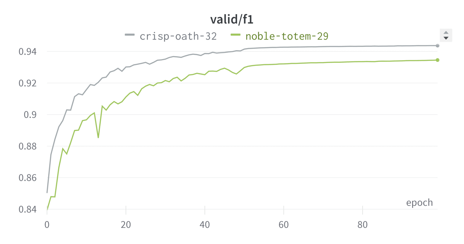
In practice, we found that using a combined loss (Dice loss + CCE loss) works better than Dice loss alone. This is also supported by our experiments:
Creating Custom LightningModule Class
The final custom class we need to create is the MedicalSegmentationModel which inherits its functionalities from Lightning’s LightningModule class.
The LightningModule class in pytorch-lightning is a higher-level abstraction that simplifies the training and organizing of PyTorch models. It provides a structured, standardized interface for defining and training deep learning models. It separates the concerns of model definition, optimization, and training loop, making the code more modular and readable.
The class methods we need to define are as follows:
- Model initialization:
__init__(...)method where the model and its parameters are defined. This method also includes the initialization of the loss and metric calculation methods. - Forward pass:
forward(...)method where the forward pass of the model is defined. - Training step:
training_step(...)method where the training step for each batch is defined. It includes calculating loss and metrics, which are logged for tracking. - Validation step:
validation_step(...)method where the validation step for each batch is defined. It also includes the calculation of loss and metrics. - Optimizer configuration:
configure_optimizers(...)method where the optimizer and, optionally, the learning rate scheduler are defined.
Moreover, two methods, on_train_epoch_end(...) and on_validation_epoch_end(...), are defined to log the average loss and f1 score after each epoch for training and validation, respectively.
class MedicalSegmentationModel(pl.LightningModule):
    def __init__(
        self,
        model_name: str,
        num_classes: int = 10,
        init_lr: float = 0.001,
        optimizer_name: str = "Adam",
        weight_decay: float = 1e-4,
        use_scheduler: bool = False,
        scheduler_name: str = "multistep_lr",
        num_epochs: int = 100,
    ):
        super().__init__()

        # Save the arguments as hyperparameters.
        self.save_hyperparameters()

        # Loading model using the function defined above.
        self.model = get_model(model_name=self.hparams.model_name, num_classes=self.hparams.num_classes)

        # Initializing the required metric objects.
        self.mean_train_loss = MeanMetric()
        self.mean_train_f1 = MulticlassF1Score(num_classes=self.hparams.num_classes, average="macro")
        self.mean_valid_loss = MeanMetric()
        self.mean_valid_f1 = MulticlassF1Score(num_classes=self.hparams.num_classes, average="macro")

    def forward(self, data):
        outputs = self.model(pixel_values=data, return_dict=True)
        upsampled_logits = F.interpolate(outputs["logits"], size=data.shape[-2:], mode="bilinear", align_corners=False)
        return upsampled_logits

    def training_step(self, batch, *args, **kwargs):
        data, target = batch
        logits = self(data)

        # Calculate Combo loss (Segmentation specific loss (Dice) + cross entropy)
        loss = dice_coef_loss(logits, target, num_classes=self.hparams.num_classes)

        self.mean_train_loss(loss, weight=data.shape[0])
        self.mean_train_f1(logits.detach(), target)

        self.log("train/batch_loss", self.mean_train_loss, prog_bar=True, logger=False)
        self.log("train/batch_f1", self.mean_train_f1, prog_bar=True, logger=False)
        return loss

    def on_train_epoch_end(self):
        # Computing and logging the training mean loss & mean f1.
        self.log("train/loss", self.mean_train_loss, prog_bar=True)
        self.log("train/f1", self.mean_train_f1, prog_bar=True)
        self.log("epoch", self.current_epoch)

    def validation_step(self, batch, *args, **kwargs):
        data, target = batch
        logits = self(data)

        # Calculate Combo loss (Segmentation specific loss (Dice) + cross entropy)
        loss = dice_coef_loss(logits, target, num_classes=self.hparams.num_classes)

        self.mean_valid_loss.update(loss, weight=data.shape[0])
        self.mean_valid_f1.update(logits, target)

    def on_validation_epoch_end(self):

        # Computing and logging the validation mean loss & mean f1.
        self.log("valid/loss", self.mean_valid_loss, prog_bar=True)
        self.log("valid/f1", self.mean_valid_f1, prog_bar=True)
        self.log("epoch", self.current_epoch)

    def configure_optimizers(self):
        optimizer = getattr(torch.optim, self.hparams.optimizer_name)(
            filter(lambda p: p.requires_grad, self.model.parameters()),
            lr=self.hparams.init_lr,
            weight_decay=self.hparams.weight_decay,
        )

        LR = self.hparams.init_lr
        WD = self.hparams.weight_decay

        if self.hparams.optimizer_name in ("AdamW", "Adam"):
            optimizer = getattr(torch.optim, self.hparams.optimizer_name)(model.parameters(), lr=LR,
                                                                          weight_decay=WD, amsgrad=True)
        else:
            optimizer = optim.SGD(model.parameters(), lr=LR, weight_decay=WD)

        if self.hparams.use_scheduler:
            lr_scheduler = torch.optim.lr_scheduler.MultiStepLR(optimizer, milestones=[self.trainer.max_epochs // 2,], gamma=0.1)

            # The lr_scheduler_config is a dictionary that contains the scheduler
            # and its associated configuration.
            lr_scheduler_config = {"scheduler": lr_scheduler, "interval": "epoch", "name": "multi_step_lr"}
            return {"optimizer": optimizer, "lr_scheduler": lr_scheduler_config}

        else:
            return optimizer
Start Training
Once we have organized the LightningModule and LightningDataModule classes, we can utilize Lightning’s Trainer class to automate the remaining tasks effortlessly.
The Trainer offers a range of valuable deep-learning training functionalities, such as mixed-precision training, distributed training, deterministic training, profiling, gradient accumulation, batch overfitting, and more. Implementing these functionalities correctly can be time-consuming, but it becomes a swift process with the Trainer class.
By initializing our MedicalSegmentationModel and MedicalSegmentationDataModule classes and passing them to the .fit(...) method of the Trainer class instance, we can promptly commence training. This streamlined approach eliminates the need to implement various training aspects manually, providing convenience and efficiency.
# Seed everything for reproducibility.
pl.seed_everything(42, workers=True)

# Intialize custom model.
model = MedicalSegmentationModel(
    model_name=TrainingConfig.MODEL_NAME,
    num_classes=DatasetConfig.NUM_CLASSES,
    init_lr=TrainingConfig.INIT_LR,
    optimizer_name=TrainingConfig.OPTIMIZER_NAME,
    weight_decay=TrainingConfig.WEIGHT_DECAY,
    use_scheduler=TrainingConfig.USE_SCHEDULER,
    scheduler_name=TrainingConfig.SCHEDULER,
    num_epochs=TrainingConfig.NUM_EPOCHS,
)

# Initialize custom data module.
data_module = MedicalSegmentationDataModule(
    num_classes=DatasetConfig.NUM_CLASSES,
    img_size=DatasetConfig.IMAGE_SIZE,
    ds_mean=DatasetConfig.MEAN,
    ds_std=DatasetConfig.STD,
    batch_size=TrainingConfig.BATCH_SIZE,
    num_workers=TrainingConfig.NUM_WORKERS,
    pin_memory=torch.cuda.is_available(),
)
Next, we will define a ModelCheckpoint and a LearningRateMonitor callback for saving the best model during training and the current learning rate of an epoch.
# Creating ModelCheckpoint callback.
# We'll save the model on basis on validation f1-score.
model_checkpoint = ModelCheckpoint(
    monitor="valid/f1",
    mode="max",
    filename="ckpt_{epoch:03d}-vloss_{valid/loss:.4f}_vf1_{valid/f1:.4f}",
    auto_insert_metric_name=False,
)

# Creating a learning rate monitor callback which will be plotted/added in the default logger.
lr_rate_monitor = LearningRateMonitor(logging_interval="epoch")
We will also initialize the WandbLogger to upload the training metrics to your wandb project. When the logger is initialized, we pass two parameters:
log_model=True– Upload the model as an artifact when the training is completed.project– The project name to use on WandB. A project typically contains logs from multiple experiments along with their trained checkpoints.
# Initialize logger.
wandb_logger = WandbLogger(log_model=True, project="UM_medical_segmentation")
When the logger is initialized, it will also print the link for the current experiment, which you open on any device to monitor the training process and also share with your team.
Train
# Initializing the Trainer class object.
trainer = pl.Trainer(
    accelerator="auto",  # Auto select the best hardware accelerator available
    devices="auto",  # Auto select available devices for the accelerator (For eg. mutiple GPUs)
    strategy="auto",  # Auto select the distributed training strategy.
    max_epochs=TrainingConfig.NUM_EPOCHS,  # Maximum number of epoch to train for.
    enable_model_summary=False,  # Disable printing of model summary as we are using torchinfo.
    callbacks=[model_checkpoint, lr_rate_monitor],  # Declaring callbacks to use.
    precision="16-mixed",  # Using Mixed Precision training.
    logger=wandb_logger
)

# Start training
trainer.fit(model, data_module)
Inference on the Medical Segmentation Dataset
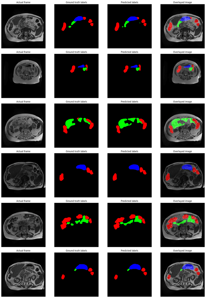
For inference, we will use the same validation data as we did during training. We will plot the ground truth images, the ground truth masks, and the predicted segmentation maps overlayed on the ground truth images.
Load The Best Trained Model
# Get the path of the best saved model.
CKPT_PATH = model_checkpoint.best_model_path
CKPT_PATH
Initialize the model with trained weights.
model = MedicalSegmentationModel.load_from_checkpoint(CKPT_PATH)
Evaluate Model On Validation Dataset
# Get the validation dataloader.

data_module.setup()
valid_loader = data_module.val_dataloader()
Get the best evaluation metrics using the saved model.
# Initialize trainer class for inference.
trainer = pl.Trainer(
    accelerator="gpu",
    devices=1,
    enable_checkpointing=False,
    inference_mode=True,
)

# Run evaluation.
results = trainer.validate(model=model, dataloaders=valid_loader)
| Validation metric | DataLoader 0 |
| valid/f1 | 0.9437294006347656 |
| valid/loss | 0.31268423795700073 |

Log them as experiment summary metrics to WandB
if os.environ.get("LOCAL_RANK", None) is None:
    wandb.run.summary["best_valid_f1"] = results[0]["valid/f1"]
    wandb.run.summary["best_valid_loss"] = results[0]["valid/loss"]
Image Inference Using DataLoader Objects
In the code below, we define a helper function that performs inference given a trained model and a dataloader object. The model prediction will also be uploaded to wandb.
@torch.inference_mode()
def inference(model, loader, img_size, device="cpu"):
    num_batches_to_process = InferenceConfig.NUM_BATCHES

    for idx, (batch_img, batch_mask) in enumerate(loader):
        predictions = model(batch_img.to(device))

        pred_all = predictions.argmax(dim=1).cpu().numpy()

        batch_img = denormalize(batch_img.cpu(), mean=DatasetConfig.MEAN, std=DatasetConfig.STD)
        batch_img = batch_img.permute(0, 2, 3, 1).numpy()

        if idx == num_batches_to_process:
            break

        for i in range(0, len(batch_img)):
            fig = plt.figure(figsize=(20, 8))

            # Display the original image.
            ax1 = fig.add_subplot(1, 4, 1)
            ax1.imshow(batch_img[i])
            ax1.title.set_text("Actual frame")
            plt.axis("off")

            # Display the ground truth mask.
            true_mask_rgb = num_to_rgb(batch_mask[i], color_map=id2color)
            ax2 = fig.add_subplot(1, 4, 2)
            ax2.set_title("Ground truth labels")
            ax2.imshow(true_mask_rgb)
            plt.axis("off")

            # Display the predicted segmentation mask.
            pred_mask_rgb = num_to_rgb(pred_all[i], color_map=id2color)
            ax3 = fig.add_subplot(1, 4, 3)
            ax3.set_title("Predicted labels")
            ax3.imshow(pred_mask_rgb)
            plt.axis("off")

            # Display the predicted segmentation mask overlayed on the original image.
            overlayed_image = image_overlay(batch_img[i], pred_mask_rgb)
            ax4 = fig.add_subplot(1, 4, 4)
            ax4.set_title("Overlayed image")
            ax4.imshow(overlayed_image)
            plt.axis("off")
            plt.show()

            # Upload predictions to WandB.
            images = wandb.Image(fig, caption=f"Prediction Sample {idx}_{i}")

            if os.environ.get("LOCAL_RANK", None) is None:
                wandb.log({"Predictions": images})
Usage:
# Use GPU if available.
DEVICE = torch.device("cuda:0") if torch.cuda.is_available() else torch.device("cpu")
model.to(DEVICE)
model.eval()

inference(model, valid_loader, device=DEVICE, img_size=DatasetConfig.IMAGE_SIZE)
Here are a few output samples.
Terminate the wandb experiment run.
if os.environ.get("LOCAL_RANK", None) is None:
    wandb.run.finish()
Building The Gradio App
Medical Image Segmentation: Next, we’ll build a small UI app using Gradio for demonstration. The app can also be easily deployed on HuggingFace spaces.
If you observe, the size of the trained checkpoint file saved by lightning is around 997 MB. It contains the model’s and optimizer’s state_dict() and additional information such as callbacks, schedulers, etc.
To make things easier and reduce the file size to be deployed, we’ve extracted the model’s state_dict() from the pytorch-lightning checkpoint and processed it such that we can directly pass it to SegformerForSemanticSegmentation.from_pretrained(…) method.
Here are the steps that we followed:
A) Checking the contents of pytorch-lightning .ckpt file.
import wandb

# Download best checkpoint file.
run = wandb.init()
artifact = run.use_artifact("veb-101/UM_medical_segmentation/model-fpgquxev:v0", type="model")
artifact_dir = artifact.download()

# Inspect checkpoint keys.
CKPT = torch.load(os.path.join(artifact_dir, "model.ckpt"), map_location="cpu")
print(CKPT.keys())

"""
dict_keys(['epoch', 'global_step', 'pytorch-lightning_version', 'state_dict', 'loops', 'callbacks', 'optimizer_states', 'lr_schedulers', 'MixedPrecisionPlugin', 'hparams_name', 'hyper_parameters'])
"""
B) Check the “key” string format for the parameter loaded using the`SegformerForSemanticSegmentation.from_pretrained(...)` method.
model = get_model(model_path=TrainingConfig.MODEL_NAME, num_classes=DatasetConfig.NUM_CLASSES)

# Get model state_dict() dictionary.
model_state_dict = model.state_dict()

# Print parmater key string.
for i, (key, val) in enumerate(model_state_dict.items()):
    print(key)
    if i == 5:
        break

"""
...
...
segformer.encoder.patch_embeddings.0.proj.weight
segformer.encoder.patch_embeddings.0.proj.bias
segformer.encoder.patch_embeddings.0.layer_norm.weight
segformer.encoder.patch_embeddings.0.layer_norm.bias
segformer.encoder.patch_embeddings.1.proj.weight
segformer.encoder.patch_embeddings.1.proj.bias
"""
Notice that each parameter key string has the prefix “segformer.”.
C) Check the same but for the pytorch-lightning checkpoint.
TRAINED_CKPT_state_dict = CKPT["state_dict"]

for i, (key, val) in enumerate(TRAINED_CKPT_state_dict.items()):
    print(key)
    if i == 5:
        break

"""
model.segformer.encoder.patch_embeddings.0.proj.weight
model.segformer.encoder.patch_embeddings.0.proj.bias
model.segformer.encoder.patch_embeddings.0.layer_norm.weight
model.segformer.encoder.patch_embeddings.0.layer_norm.bias
model.segformer.encoder.patch_embeddings.1.proj.weight
model.segformer.encoder.patch_embeddings.1.proj.bias
"""
And here we see the difference between the parameter key strings. The extra “model.” prefix is the name of the variable used inside the MedicalSegmentationModel class to hold the model.
D) To remove the dependency on pytorch-lightning during inference, we will create a new state_dict() dictionary object where the keys will be the same as the ones in step B and the values will be from the pytorch-lightning checkpoint.
from collections import OrderedDict

new_state_dict = OrderedDict()

for key_name, value in CKPT["state_dict"].items():
    new_state_dict[key_name.replace("model.", "")] = value

# Check
model = get_model(model_path=TrainingConfig.MODEL_NAME, num_classes=DatasetConfig.NUM_CLASSES)

model.load_state_dict(new_state_dict)

"""
<All keys matched successfully>
"""
E) Next, we’ll use the .save_pretrained(...) method to save the transformer model.
# Saves model's configuration and weights in "segformer_trained_weights" directory.
model.save_pretrained("segformer_trained_weights")
So the next time we want to load the trained Segformer model, we can simply do:
# Pass the location of  "segformer_trained_weights" directory
# instead of ""nvidia/segformer-b4-finetuned-ade-512-512"

model = get_model(model_path="segformer_trained_weights", num_classes=DatasetConfig.NUM_CLASSES)
The size of the new file is just 224 MB which is significantly smaller. This will also help to load the model quickly, as we are only loading the model’s parameters.
Script: app.py
The majority of the code remains the same. The only new function is the predict(…). It takes in a Pillow image and returns a list of tuples of length three (one for each class). The tuple object at each index contains 2 elements. One is the binary segmentation mask for the class, and the second is the class name. This output format is required by the gr.AnnotatedImage(...) component to display the image with predicted mask overlays.
import os
import numpy as np
import gradio as gr
from glob import glob
from functools import partial
from dataclasses import dataclass

import torch
import torch.nn.functional as F
import torchvision.transforms as TF
from transformers import SegformerForSemanticSegmentation


@dataclass
class Configs:
    NUM_CLASSES: int = 4  # including background.
    CLASSES: tuple = ("Large bowel", "Small bowel", "Stomach")
    IMAGE_SIZE: tuple[int, int] = (288, 288)  # W, H
    MEAN: tuple = (0.485, 0.456, 0.406)
    STD: tuple = (0.229, 0.224, 0.225)
    MODEL_PATH: str = os.path.join(os.getcwd(), "segformer_trained_weights")


def get_model(*, model_path, num_classes):
    model = SegformerForSemanticSegmentation.from_pretrained(model_path, num_labels=num_classes, ignore_mismatched_sizes=True)
    return model


@torch.inference_mode()
def predict(input_image, model=None, preprocess_fn=None, device="cpu"):
    shape_H_W = input_image.size[::-1]
    input_tensor = preprocess_fn(input_image)
    input_tensor = input_tensor.unsqueeze(0).to(device)

    # Generate predictions
    outputs = model(pixel_values=input_tensor.to(device), return_dict=True)
    predictions = F.interpolate(outputs["logits"], size=shape_H_W, mode="bilinear", align_corners=False)

    preds_argmax = predictions.argmax(dim=1).cpu().squeeze().numpy()

    seg_info = [(preds_argmax == idx, class_name) for idx, class_name in enumerate(Configs.CLASSES, 1)]

    return (input_image, seg_info)


if __name__ == "__main__":
    class2hexcolor = {"Stomach": "#007fff", "Small bowel": "#009A17", "Large bowel": "#FF0000"}

    DEVICE = torch.device("cuda:0") if torch.cuda.is_available() else torch.device("cpu")

    model = get_model(model_path=Configs.MODEL_PATH, num_classes=Configs.NUM_CLASSES)
    model.to(DEVICE)
    model.eval()
    _ = model(torch.randn(1, 3, *Configs.IMAGE_SIZE[::-1], device=DEVICE))

    preprocess = TF.Compose(
        [
            TF.Resize(size=Configs.IMAGE_SIZE[::-1]),
            TF.ToTensor(),
            TF.Normalize(Configs.MEAN, Configs.STD, inplace=True),
        ]
    )

    with gr.Blocks(title="Medical Image Segmentation") as demo:
        gr.Markdown("""<h1><center>Medical Image Segmentation with UW-Madison GI Tract Dataset</center></h1>""")
        with gr.Row():
            img_input = gr.Image(type="pil", height=360, width=360, label="Input image")
            img_output = gr.AnnotatedImage(label="Predictions", height=360, width=360, color_map=class2hexcolor)

        section_btn = gr.Button("Generate Predictions")
        section_btn.click(partial(predict, model=model, preprocess_fn=preprocess, device=DEVICE), img_input, img_output)

        images_dir = glob(os.path.join(os.getcwd(), "samples") + os.sep + "*.png")
        examples = [i for i in np.random.choice(images_dir, size=8, replace=False)]
        gr.Examples(examples=examples, inputs=img_input, outputs=img_output)

    demo.launch()
You can use the Gradio inference demo here –> Medical Image Segmentation Gradio App
All the files required can be accessed from here –> Gradio App Files
You can also try out the Gradio app embedded below.
Summary
Medical image segmentation using deep learning provides significant advantages. Deep learning models excel at capturing complex patterns and features, leading to highly accurate and precise segmentation results compared to traditional methods. Additionally, deep learning algorithms automate segmentation, improving efficiency and enabling analysis of large volumes of medical image data. Moreover, deep learning models demonstrate adaptability and generalization, making them suitable for diverse image characteristics, imaging modalities, patient populations, and clinical settings, expanding their utility in medical imaging applications.
To summarise this article📜, we covered a comprehensive list of related topics:
- Medical Image Segmentation: Explored the definition and challenges of medical image segmentation.
- Dataset Preparation: Used the UW-Madison GI Tract segmentation dataset, made observations, and created preprocessed training and validation sets.
- We defined a few essential functions and classes for PyTorch and PyTorch-Lightning frameworks to facilitate ease of training.
- We learned how to use the Segformer model from Hugging Face transformers for segmentation and fine-tuned it on our dataset.
- We defined a custom loss function combining the Dice coefficient with cross-entropy for improved segmentation performance.
- Training and Metrics Tracking: Trained the model, monitored metrics using WandB, and uploaded the model as an artifact for future use.
- We designed a user-friendly interface using the Gradio app, making our medical multi-label image classification model accessible to everyone.
References
- UWM – GI Tract Image Segmentation – EDA
- ⚕️ AW-Madison: EDA & In Depth Mask Exploration
- UWMGI: Unet [Train] [PyTorch]


