Introduction to Video Classification and Human Activity Recognition

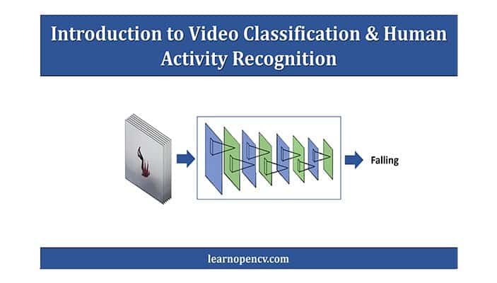
In this post, we will learn about Video Classification. We will go over a number of approaches to make a video classifier for Human Activity Recognition. Basically, you will learn video classification and human activity recognition.

Outline:

Here’s an outline for this post.

1. Understanding Human Activity Recognition.
2. Video Classification and Human Activity Recognition – Introduction.
3. Video Classification Methods.
4. Types of Video Classification problems.
5. Making a Video Classifier Using Keras. (Moving Average and Single Frame-CNN)
6. Summary

1: Understanding Human Activity Recognition

Before we talk about Video Classification, let us first understand what Human Activity Recognition is.

To put it simply, the task of classifying or predicting the activity/action being performed by someone is called Activity recognition.

We may have a question here: how is this different from a normal Classification task? The thing here is, in Human Activity Recognition, you actually need a series of data points to predict the action being performed correctly.

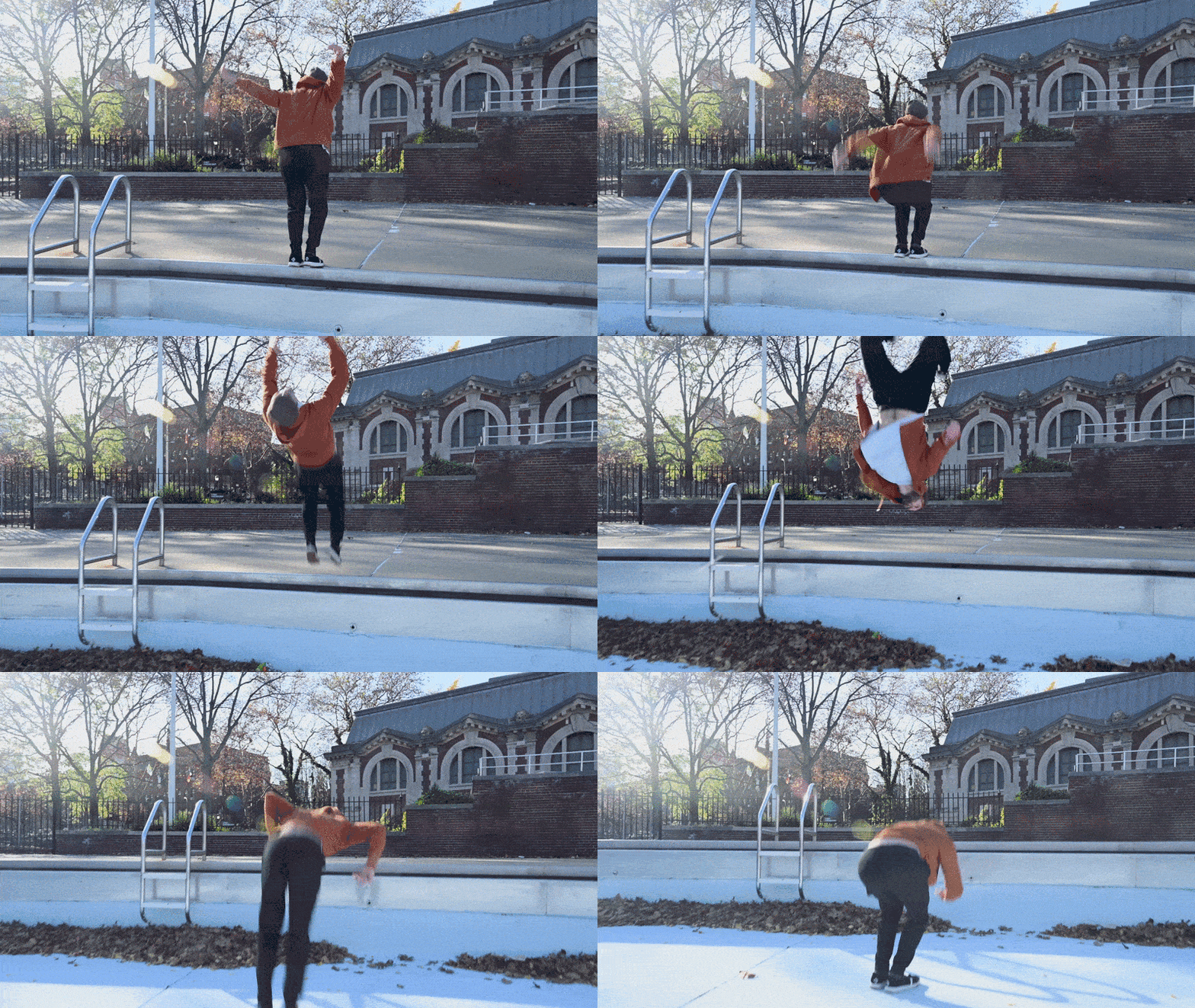
Take a look at this backflip action done by this person, we can only tell it is a backflip by watching the full video.

If we were to provide a model with just a random snapshot (like the image below) from the video clip above then it might predict the action incorrectly.

If a model sees only the above image, then it kind of looks like the person is falling so it predicts falling.

So Human Activity Recognition is a type of time series classification problem where you need data from a series of timesteps to correctly classify the action being performed.

So how was Human Activity Recognition traditionally solved?

The most common and effective technique is to attach a wearable sensor (example a smartphone) on to a person and then train a temporal model like an LSTM on the output of the sensor data. 

For example take a look at this Video:

Here the person’s movement in x,y,z is the direction and his angular velocity is being recorded by the accelerometer and the gyroscope sensor in the smartphone.

A model is then trained on this sensor data to output these six classes.

1. Walking
2. Walking Upstairs
3. Walking Downstairs
4. Sitting
5. Standing
6. Laying

You can download the dataset here.

This approach to activity recognition is remarkably effective. This video is actually a part of a dataset called ‘Activity Recognition Using Smartphones‘. It was prepared and made available by Davide Anguita, et al. from the University of Genova, Italy.      The details are available in their 2013 paper “A Public Domain Dataset for Human Activity Recognition Using Smartphones.”

But in this post we are not going to train a model on sensor data, for two reasons:

1. In most practical scenarios you won’t have access to sensor data. For example, if you want to detect Illegal Activity at a place then you may have to rely on just video feeds from CCTV cameras.

2. I am mostly interested in solving this problem using Computer Vision, so we will be using Video Classification methods to achieve activity recognition.

Note: If you’re interested in using sensor data to predict activity then you can take a look at this post by Jason Brownlee from machinelearningmastery.

2: Video Classification And Human Activity Recognition – Introduction

Now that we have established the need for Video Classification models to solve the problem of Human Activity Recognition, let us discuss the most basic and naive approach for Video Classification.

Here is the Good News, if you have some experience building basic image classification models then you can already create a great video classification system.

Consider this demo, where we are using a normal classification model to predict each individual frame of the video, and the results are surprisingly good.

How is that possible?

But just a few moments ago, I showed you with that backflip example that for activity recognition, you cannot rely on a single frame, so why is a simple classification model performing so well?

Here is the thing:

The model is also learning the environmental context. Consider example below.

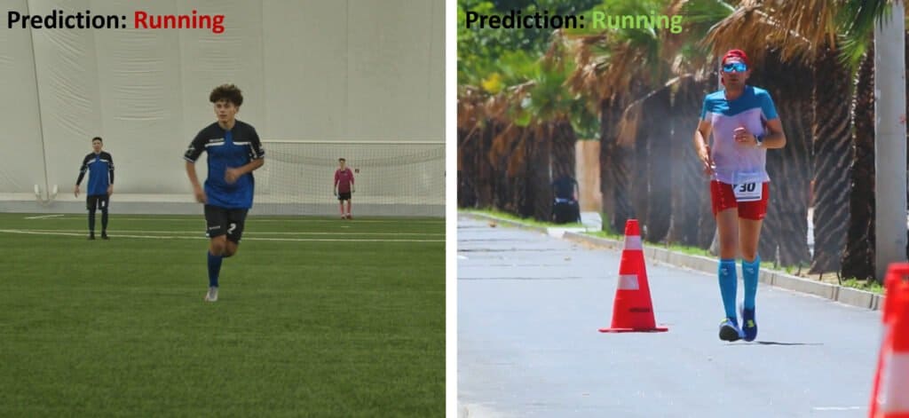
Normally both images below will be classified as running by an image classifier.

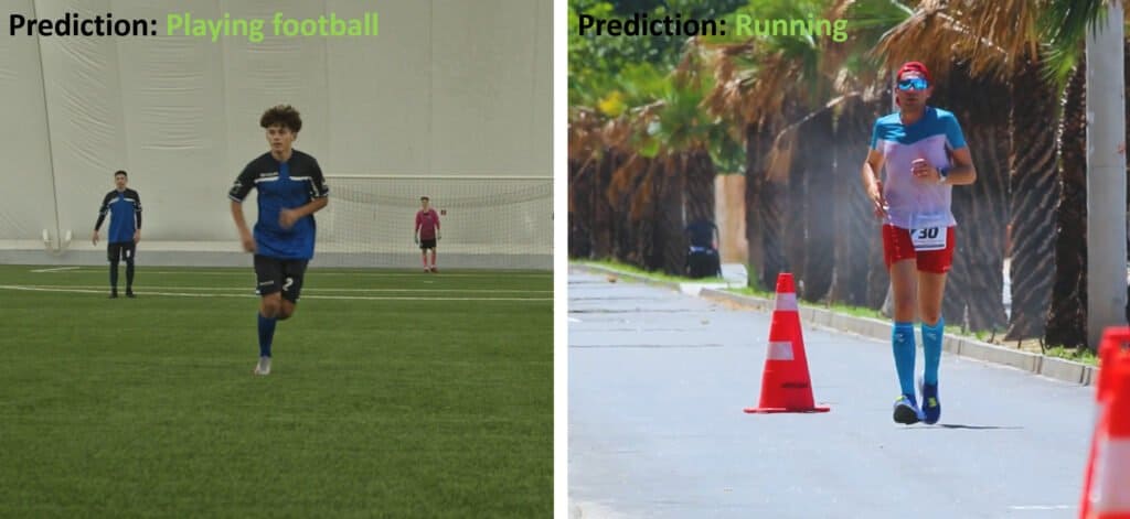
But with enough examples like below:

The model learns to distinguish between two similar actions by using environmental context.

So with enough examples, the model learns that a person with a running pose on a football field is most likely to be playing football, and if the person with that pose is on a track or a road then he’s probably running. 

Now there is a drawback with this approach.

The issue is that the model will not always be fully confident about each video frame’s prediction, so the predictions will change rapidly and fluctuate.

This is because the model is not looking at the entire video sequence but just classifying each frame independently.

An easy solution to this problem is instead of classifying and displaying results for a single frame, why not average results over 5, 10, or n frames. This would effectively get rid of that flickering.

Once we have decided on the value of n, we can then use something as simple as the moving average/rolling average technique to achieve this.

So suppose:

n = Number of frames to average over

P_f = Final predicted probabilities

P =  Current frame’s predicted probabilities

P_-1 = Last frame’s predicted probabilities

P_-2 = 2^nd last frame’s predicted probabilities

.

.

P_-n+1 = (n-1)^th last frame’s predicted probabilities

So here is how you calculate moving average:

So if you had n=3 and had two classes running and walking then:

The predicted values are:

, ,

Putting values in the formula:

As 0.97 (Running score) > 0.03 (Walking score), so Prediction = Running.

So by just utilizing the above formula you will get rid of the flickering.

In this tutorial, we will cover how to train a model with moving average in Keras.

However, it’s worth mentioning that these two approaches are not actual Video Classification methods but merely hacks. (Which are effective).

But here is the problem,

Depending upon the model to learn environmental context instead of the actual action sequence to predict is terribly wrong and it will lead to over fitting.

This is also the reason the approaches above will not work well when the actions are similar.

Consider the action of Standing Up from a Chair and Sitting Down on a Chair. In both actions, the frames are almost the same. The main differentiator is the order of the frame sequence. So you need temporal information to correctly predict these actions.

Now, there are some robust video classification methods that utilize the temporal information in a video and solves for the above issues.

3. Video Classification Methods:

In this section we will take a look at some methods to perform video classification, we are looking at methods that can take input, a short video clip and then output the Activity being performed in that video clip.

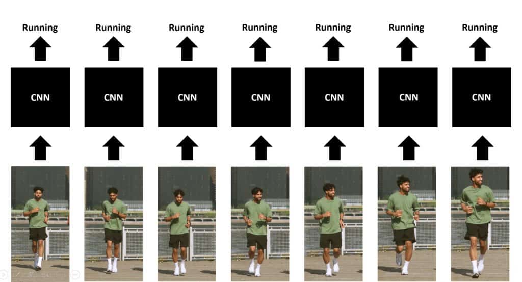
Method 1: Single-Frame CNN:

We have already established that the most basic implementation of video classification is using an image classification network. Now, we will run an image classification model on every single frame of the video and then average all the individual probabilities to get the final probabilities vector. This approach does perform really well, and we will get to implement it in this post.

Also, it is worth mentioning that videos generally contain a lot of frames, and we do not need to run a classification model on each frame, but only a few of them that are spread out throughout the entire video.

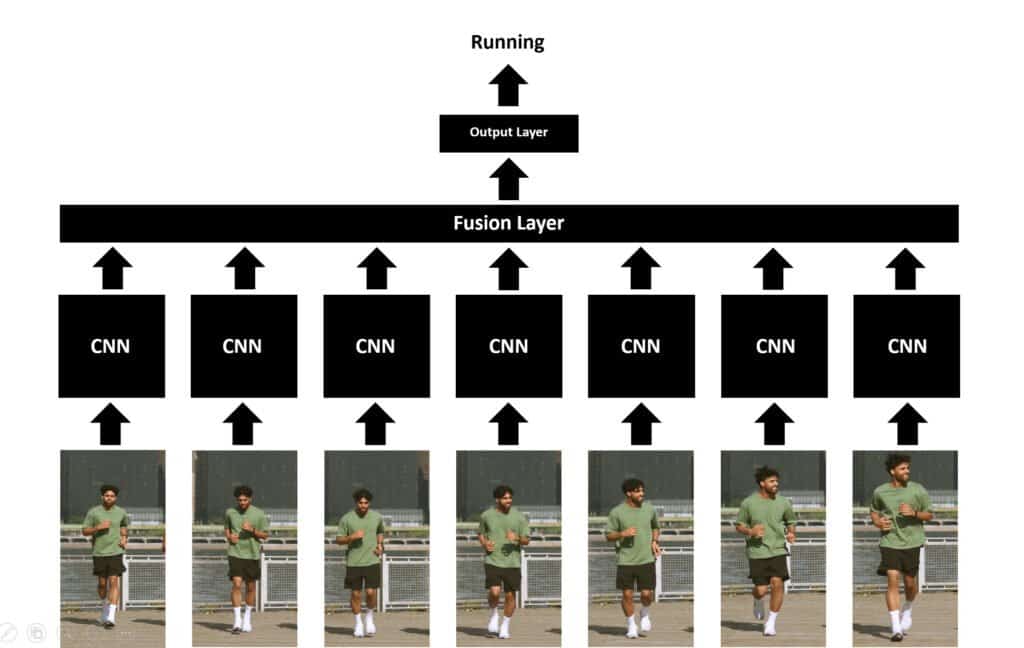
Method 2: Late Fusion:

The Late Fusion approach, in practice, is very similar to the Single-Frame CNN approach but slightly more complicated. The only difference is that in the Single-Frame CNN approach, averaging across all the predicted probabilities is performed once the network has finished its work, but in the Late Fusion approach, the process of averaging (or some other fusion technique) is built into the network itself. Due to this, the temporal structure of the frames sequence is also taken into account.

A Fusion layer is used to merge the output of separate networks that operate on temporally distant frames. It is normally implemented using the max pooling, average pooling or flattening technique.

This approach enables the model to learn spatial as well as temporal information about the appearance and movement of the objects in a scene. Each stream performs image (frame) classification on its own, and in the end, the predicted scores are merged using the fusion layer.

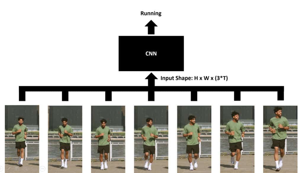
Method 3: Early Fusion:

This approach is opposite of the late fusion, as, in this approach, the temporal dimension and the channel (RGB) dimension of the video are fused at the start before passing it to the model which allows the first layer to operate over frames and learn to identify local pixel motions between adjacent frames.

An input video of shape (T x 3 x H x W) with a temporal dimension, three RGB channel dimensions, and two spatial dimensions H and W, after fusion, becomes a tensor of shape (3T x H x W). 

Method 4: Using CNN with LSTM’s:

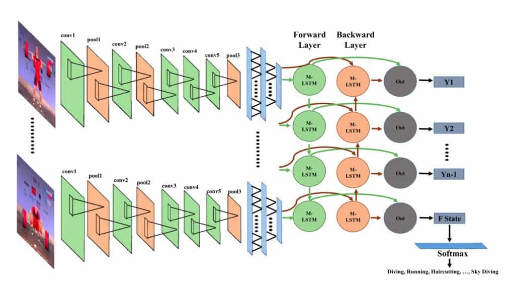
The idea in this approach is to use convolutional networks to extract local features of each frame. The outputs of these independent convolutional networks are fed to a many-to-one multilayer LSTM network to fuse this extracted information temporarily.

You can read the paper “Action Recognition in Video Sequences using Deep Bi-Directional LSTM With CNN Features”, by Amin Ullah (IEEE 2017),     to learn more about this approach.

Method 5: Using Pose Detection and LSTM:

Another interesting idea is to use an off the shelf pose detection model to get the key points of a person’s body  for each frame in the video and then use those extracted key points and feed them to an LSTM network to determine the activity being performed in the video. 

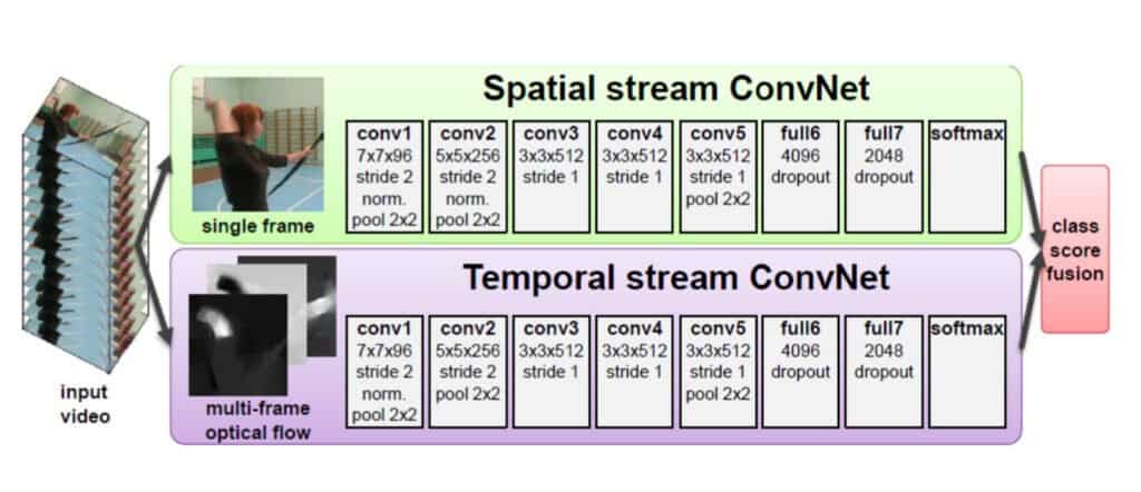
Method 6: Using Optical Flow and CNN’s:

Optical flow is the pattern of visible motion of objects, edges and helps calculate the motion vector of every pixel in a video frame. It is effectively used in motion tracking applications. So why not combine this with a CNN to capture motion      and spatial context in a video. The paper titled “A Comprehensive Review on Handcrafted and Learning-Based Action Representation Approaches for Human Activity Recognition”, by Allah Bux Sargano (2017), provides such an approach.

In this approach, two parallel streams of convolutional networks are used. The steam on top is known as Spatial Stream. It takes a single frame from the video and then runs a bunch of CNN kernels on it, and then based on its spatial information it makes a prediction.

The stream on the bottom called the Temporal stream takes every adjacent frame’s optical flows after merging them using the early fusion technique and then using the motion information to make a prediction. In the end, the averaging across both predicted probabilities is performed to get the final probabilities.    

The problem with this approach is that it relies on an external optical flow algorithm outside of the main network to find optical flows for each video.

Method 7: Using SlowFast Networks:

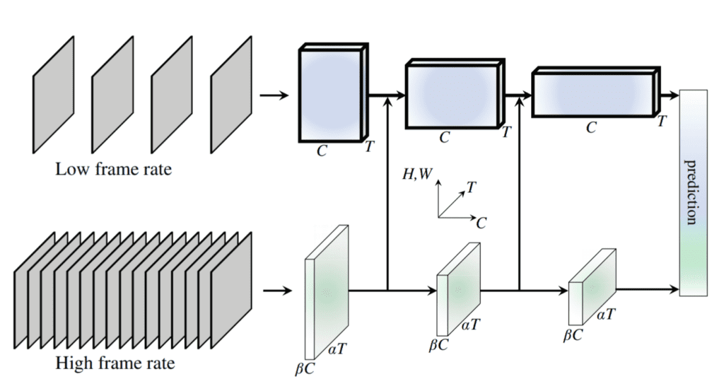
Similar to the previous method this approach also has two parallel streams. One stream operates on a temporarily low resolution video compared to the other. All operations temporal and spatial are done in a single network.

The stream on top, called the slow branch, operates on a low temporal frame rate video and has a lot of channels at every layer for detailed processing for each frame. On the other hand, the stream on the bottom, also known as the fast branch, has low channels and operates on a high temporal frame rate version of the same video. 

Both streams are connected to merge the information from the fast branch to the slow branch at multiple stages. For more details and insight into this approach, read this paper, “SlowFast Networks for Video Recognition” by Christoph Feichtenhofer ( ICCV 2019).

Method 8: Using 3D CNN’s / Slow Fusion :

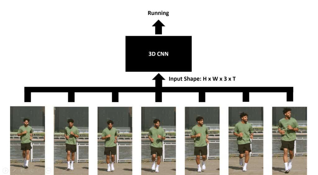
This approach uses a 3D convolution network that allows you to process temporal information and spatial by using a 3 Dimensional CNN. This method is also called the  Slow Fusion approach. Unlike Early and Late fusion, this method fuses the temporal and spatial information slowly at each CNN layer throughout the entire network.

A four-dimensional tensor (two spatial dimensions, one channel dimension and one temporal dimension) of shape H W C T is passed through the model, allowing it to easily learn all types of temporal interactions between adjacent frames.

A drawback with this approach is that increasing the input dimensions also tremendously increases the computational and memory requirements. The paper titled “3D Convolutional Neural Networks for Human Action Recognition”, by Shuiwang Ji (IEEE 2012), provides a detailed explanation of this approach. 

A paper named “Large-scale Video Classification with Convolutional Neural Networks”  by Andrej Karpathy (CVPR 2014), provides an excellent comparison between some of the methods mentioned above. 

4: Types of Activity Recognition Problems:

We have looked at various model architectural types used to perform video classification. Now let us take a look at the types of activity recognition problems out there in the context of video classification.

So the task of performing activity recognition in a video can be broken down into 3 broad categories. Please note this is not some official categorization, but it is how I would personally break it down.

Simple Activity Recognition: 

In this type, we have a model that takes in a short video clip and classifies the singular global action being performed. All the methods discussed in the previous section fall into this category.

Temporal Activity Recognition/Localization:

Suppose we have a long video that contains not one but multiple actions at different time intervals. What would we do then?

In such cases, we can use an approach called Temporal Activity localization. The model has an architecture containing two parts. The first part localizes each individual action into temporal proposals. Then the second part classifies each video clip/proposal.

The methodology is similar to Faster RCNN, generate proposals and then classify. You can read this excellent paper called “Rethinking the Faster R-CNN Architecture for Temporal Action Localization” (CVPR 2018)  by Yu-Wei Chao to learn more about this problem.

Spatio-Temporal Detection:

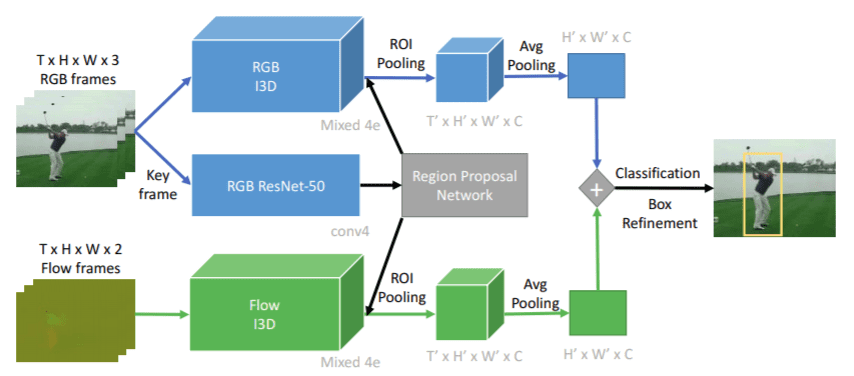
Another type of problem similar to the previous one is when we have a video containing multiple people. All of them are performing different actions. We have to detect and localize each person in the video and classify activities being performed by each individual. Plus, we also need to make a note of the time span of each action being performed, just like in temporal activity recognition. This problem is called Spatio-Temporal Detection.

As we can see, this is a tough and challenging problem. This paper, “AVA: A Video Dataset of Spatio-temporally Localized Atomic Visual Actions”, (CVPR 2018) by Chunhui Gu introduces a great dataset for researchers to train models for this problem.

5: Video Classification Using Keras:

Alright, now enough with the theory. Let us create a basic video classification system with Keras. We will first create a normal classifier, then implement a moving average technique and then finally create a Single Frame CNN video classifier.

Also, it is worth mentioning that Adrian Rosebrock from pyimagesearch has also published an interesting tutorial on Video Classification here.

Here are the steps we will perform:

• Step 1: Download and Extract the Dataset
• Step 2: Visualize the Data with its Labels
• Step 3: Read and Preprocess the Dataset
• Step 4: Split the Data into Train and Test Set
• Step 5: Construct the Model
• Step 6: Compile and Train the Model
• Step 7: Plot Model’s Loss and Accuracy Curves
• Step 8: Make Predictions with the Model
• Step 9: Using Single-Frame CNN Method

Make sure you have pafy, youtube-dl and moviepy packages installed.

!pip install pafy youtube-dl moviepy

Import Required Libraries:

Click here to download the source code to this post

Start by importing all required libraries.

import os
import cv2
import math
import pafy
import random
import numpy as np
import datetime as dt
import tensorflow as tf
from moviepy.editor import *
from collections import deque
import matplotlib.pyplot as plt
%matplotlib inline

from sklearn.model_selection import train_test_split

from tensorflow.keras.layers import *
from tensorflow.keras.models import Sequential
from tensorflow.keras.utils import to_categorical
from tensorflow.keras.callbacks import EarlyStopping
from tensorflow.keras.utils import plot_model

Set Numpy, Python and Tensorflow seeds to get consistent results.

seed_constant = 23
np.random.seed(seed_constant)
random.seed(seed_constant)
tf.random.set_seed(seed_constant)

Step 1: Download and Extract the Dataset

Let us start by downloading the dataset.

The Dataset we are using is the UCF50 – Action Recognition Dataset.

UCF50 is an action recognition dataset which contains:

• 50 Action Categories consisting of realistic YouTube videos
• 25 Groups of Videos per Action Category
• 133 Average Videos per Action Category
• 199 Average Number of Frames per Video
• 320 Average Frames Width per Video
• 240 Average Frames Height per Video
• 26 Average Frames Per Seconds per Video

After downloading the data, you will need to extract it.

!wget -nc --no-check-certificate https://www.crcv.ucf.edu/data/UCF50.rar
!unrar x UCF50.rar -inul -y

--2021-02-01 05:58:40--  https://www.crcv.ucf.edu/data/UCF50.rar
Resolving www.crcv.ucf.edu (www.crcv.ucf.edu)... 132.170.214.127
Connecting to www.crcv.ucf.edu (www.crcv.ucf.edu)|132.170.214.127|:443... connected.
WARNING: cannot verify www.crcv.ucf.edu's certificate, issued by ‘CN=InCommon RSA Server CA,OU=InCommon,O=Internet2,L=Ann Arbor,ST=MI,C=US’:
  Unable to locally verify the issuer's authority.
HTTP request sent, awaiting response... 200 OK
Length: 3233554570 (3.0G) [application/rar]
Saving to: ‘UCF50.rar’

UCF50.rar           100%[===================>]   3.01G  33.5MB/s    in 50s     

2021-02-01 05:59:30 (61.8 MB/s) - ‘UCF50.rar’ saved [3233554570/3233554570]

Step 2: Visualize the Data with its Labels

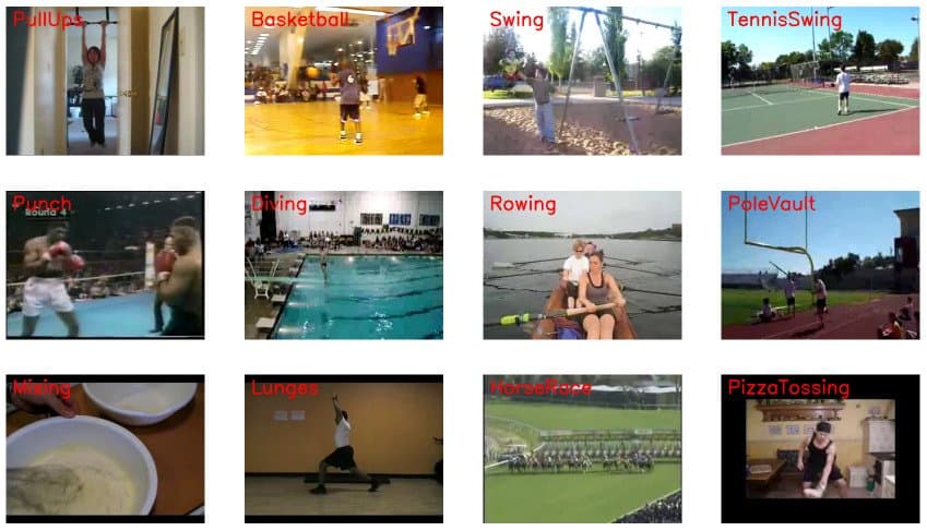
Let us pick some random videos from each class of the dataset and display it, this will give us a good overview of how the dataset looks like.

# Create a Matplotlib figure
plt.figure(figsize = (30, 30))

# Get Names of all classes in UCF50
all_classes_names = os.listdir('UCF50')

# Generate a random sample of images each time the cell runs
random_range = random.sample(range(len(all_classes_names)), 20)

# Iterating through all the random samples
for counter, random_index in enumerate(random_range, 1):

    # Getting Class Name using Random Index
    selected_class_Name = all_classes_names[random_index]

    # Getting a list of all the video files present in a Class Directory
    video_files_names_list = os.listdir(f'UCF50/{selected_class_Name}')

    # Randomly selecting a video file
    selected_video_file_name = random.choice(video_files_names_list)

    # Reading the Video File Using the Video Capture
    video_reader = cv2.VideoCapture(f'UCF50/{selected_class_Name}/{selected_video_file_name}')
    
    # Reading The First Frame of the Video File
    _, bgr_frame = video_reader.read()

    # Closing the VideoCapture object and releasing all resources. 
    video_reader.release()

    # Converting the BGR Frame to RGB Frame 
    rgb_frame = cv2.cvtColor(bgr_frame, cv2.COLOR_BGR2RGB)

    # Adding The Class Name Text on top of the Video Frame.
    cv2.putText(rgb_frame, selected_class_Name, (10, 30), cv2.FONT_HERSHEY_SIMPLEX, 1, (255, 0, 0), 2)
    
    # Assigning the Frame to a specific position of a subplot
    plt.subplot(5, 4, counter)
    plt.imshow(rgb_frame)
    plt.axis('off')

Step 3: Read and Preprocess the Dataset

Since we are going to use a classification architecture to train on a video classification dataset, we are going to need to preprocess the dataset first.

Now w constants,

• image_height and image_weight: This is the size we will resize all frames of the video to, we are doing this to avoid unnecessary computation.
• max_images_per_class: Maximum number of training images allowed for each class.
• dataset_directory: The path of the directory containing the extracted dataset.
• classes_list: These are the list of classes we are going to be training on, we are training on following 4 classes, you can feel free to change it.
  • tai chi
  • Swinging
  • Horse Racing
  • Walking with a Dog

Note: The image_height, image_weight and max_images_per_class constants may be increased for better results, but be warned this will become computationally expensive.

image_height, image_width = 64, 64
max_images_per_class = 8000

dataset_directory = "UCF50"
classes_list = ["WalkingWithDog", "TaiChi", "Swing", "HorseRace"]

model_output_size = len(classes_list)

Extract, Resize and Normalize Frames

Now we will create a function that will extract frames from each video while performing other preprocessing operation like resizing and normalizing images.

This method takes a video file path as input. It then reads the video file frame by frame, resizes each frame, normalizes the resized frame, appends the normalized frame into a list, and then finally returns that list.

def frames_extraction(video_path):
    # Empty List declared to store video frames
    frames_list = []
    
    # Reading the Video File Using the VideoCapture
    video_reader = cv2.VideoCapture(video_path)

    # Iterating through Video Frames
    while True:

        # Reading a frame from the video file 
        success, frame = video_reader.read() 

        # If Video frame was not successfully read then break the loop
        if not success:
            break

        # Resize the Frame to fixed Dimensions
        resized_frame = cv2.resize(frame, (image_height, image_width))
        
        # Normalize the resized frame by dividing it with 255 so that each pixel value then lies between 0 and 1
        normalized_frame = resized_frame / 255
        
        # Appending the normalized frame into the frames list
        frames_list.append(normalized_frame)
    
    # Closing the VideoCapture object and releasing all resources. 
    video_reader.release()

    # returning the frames list 
    return frames_list

Dataset Creation

Now we will create another function called create_dataset(), this function uses the frame_extraction() function above and creates our final preprocessed dataset.

Here’s how this function works:

1. Iterate through all the classes mentioned in the classes_list
2. Now for each class iterate through all the video files present in it.
3. Call the frame_extraction method on each video file.
4. Add the returned frames to a list called temp_features
5. After all videos of a class are processed, randomly select video frames (equal to max_images_per_class) and add them to the list called features.
6. Add labels of the selected videos to the `labels` list.
7. After all videos of all classes are processed then return the features and labels as NumPy arrays.

So when you call this function, it returns two lists:

• A list of feature vectors
• A list of its associated labels.

def create_dataset():

    # Declaring Empty Lists to store the features and labels values.
    temp_features = [] 
    features = []
    labels = []
    
    # Iterating through all the classes mentioned in the classes list
    for class_index, class_name in enumerate(classes_list):
        print(f'Extracting Data of Class: {class_name}')
        
        # Getting the list of video files present in the specific class name directory
        files_list = os.listdir(os.path.join(dataset_directory, class_name))

        # Iterating through all the files present in the files list
        for file_name in files_list:

            # Construct the complete video path
            video_file_path = os.path.join(dataset_directory, class_name, file_name)

            # Calling the frame_extraction method for every video file path
            frames = frames_extraction(video_file_path)

            # Appending the frames to a temporary list.
            temp_features.extend(frames)
        
        # Adding randomly selected frames to the features list
        features.extend(random.sample(temp_features, max_images_per_class))

        # Adding Fixed number of labels to the labels list
        labels.extend([class_index] * max_images_per_class)
        
        # Emptying the temp_features list so it can be reused to store all frames of the next class.
        temp_features.clear()

    # Converting the features and labels lists to numpy arrays
    features = np.asarray(features)
    labels = np.array(labels)  

    return features, labels

Calling the create_dataset method which returns features and labels.

features, labels = create_dataset()

Extracting Data of Class: WalkingWithDog
Extracting Data of Class: TaiChi
Extracting Data of Class: Swing
Extracting Data of Class: HorseRace

Now we will convert class labels to one hot encoded vectors.

# Using Keras's to_categorical method to convert labels into one-hot-encoded vectors
one_hot_encoded_labels = to_categorical(labels)

Step 4: Split the Data into Train and Test Sets

Now we have two numpy arrays, one containing all images. The second one contains all class labels in one hot encoded format. Let us split our data to create a training, and a testing set. We must shuffle the data before the split, which we have already done.

features_train, features_test, labels_train, labels_test = train_test_split(features, one_hot_encoded_labels, test_size = 0.2, shuffle = True, random_state = seed_constant)

Step 5: Construct the Model

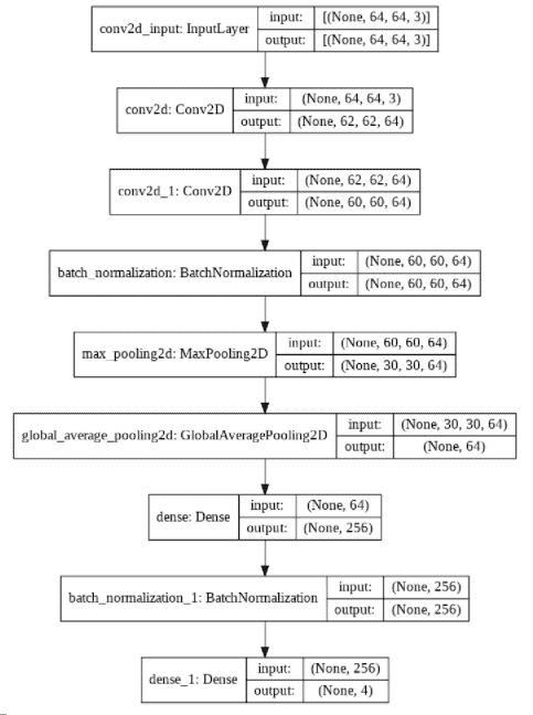
Now it is time to create our CNN model, for this post, we are creating a simple CNN Classification model with two CNN layers.

# Let's create a function that will construct our model
def create_model():

    # We will use a Sequential model for model construction
    model = Sequential()

    # Defining The Model Architecture
    model.add(Conv2D(filters = 64, kernel_size = (3, 3), activation = 'relu', input_shape = (image_height, image_width, 3)))
    model.add(Conv2D(filters = 64, kernel_size = (3, 3), activation = 'relu'))
    model.add(BatchNormalization())
    model.add(MaxPooling2D(pool_size = (2, 2)))
    model.add(GlobalAveragePooling2D())
    model.add(Dense(256, activation = 'relu'))
    model.add(BatchNormalization())
    model.add(Dense(model_output_size, activation = 'softmax'))

    # Printing the models summary
    model.summary()

    return model


# Calling the create_model method
model = create_model()

print("Model Created Successfully!")

Model: "sequential"
_________________________________________________________________
Layer (type)                 Output Shape              Param #   
=================================================================
conv2d (Conv2D)              (None, 62, 62, 64)        1792      
_________________________________________________________________
conv2d_1 (Conv2D)            (None, 60, 60, 64)        36928     
_________________________________________________________________
batch_normalization (BatchNo (None, 60, 60, 64)        256       
_________________________________________________________________
max_pooling2d (MaxPooling2D) (None, 30, 30, 64)        0         
_________________________________________________________________
global_average_pooling2d (Gl (None, 64)                0         
_________________________________________________________________
dense (Dense)                (None, 256)               16640     
_________________________________________________________________
batch_normalization_1 (Batch (None, 256)               1024      
_________________________________________________________________
dense_1 (Dense)              (None, 4)                 1028      
=================================================================
Total params: 57,668
Trainable params: 57,028
Non-trainable params: 640
_________________________________________________________________
Model Created Successfully!

Check Model’s Structure:

Using the plot_model function, we can check the structure of the final model. This is really helpful when we are creating a complex network, and you want to make sure we have constructed the network correctly.

plot_model(model, to_file = 'model_structure_plot.png', show_shapes = True, show_layer_names = True)

Step 6: Compile and Train the Model

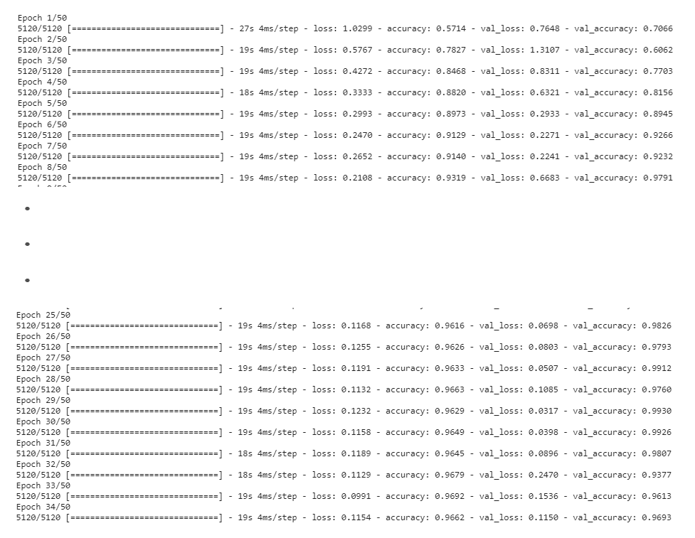
Now let us start the training. Before we do that, we also need to compile the model.

# Adding Early Stopping Callback
early_stopping_callback = EarlyStopping(monitor = 'val_loss', patience = 15, mode = 'min', restore_best_weights = True)

# Adding loss, optimizer and metrics values to the model.
model.compile(loss = 'categorical_crossentropy', optimizer = 'Adam', metrics = ["accuracy"])

# Start Training
model_training_history = model.fit(x = features_train, y = labels_train, epochs = 50, batch_size = 4 , shuffle = True, validation_split = 0.2, callbacks = [early_stopping_callback])

Evaluating Your Trained Model

Evaluate your trained model on the feature’s and label’s test sets.

model_evaluation_history = model.evaluate(features_test, labels_test)

model_evaluation_history = model.evaluate(features_test, labels_test)

200/200 [==============================] - 1s 5ms/step - loss: 0.0313 - accuracy: 0.9941

Save Your Model

You should now save your model for future runs.

# Creating a useful name for our model, incase you're saving multiple models (OPTIONAL)
date_time_format = '%Y_%m_%d__%H_%M_%S'
current_date_time_dt = dt.datetime.now()
current_date_time_string = dt.datetime.strftime(current_date_time_dt, date_time_format)
model_evaluation_loss, model_evaluation_accuracy = model_evaluation_history
model_name = f'Model___Date_Time_{current_date_time_string}___Loss_
{model_evaluation_loss}___Accuracy_{model_evaluation_accuracy}.h5'

# Saving your Model
model.save(model_name)

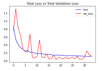
Step 7: Plot Model’s Loss and Accuracy Curves

Let us plot our loss and accuracy curves.

def plot_metric(metric_name_1, metric_name_2, plot_name):
  # Get Metric values using metric names as identifiers
  metric_value_1 = model_training_history.history[metric_name_1]
  metric_value_2 = model_training_history.history[metric_name_2]

  # Constructing a range object which will be used as time 
  epochs = range(len(metric_value_1))
  
  # Plotting the Graph
  plt.plot(epochs, metric_value_1, 'blue', label = metric_name_1)
  plt.plot(epochs, metric_value_2, 'red', label = metric_name_2)
  
  # Adding title to the plot
  plt.title(str(plot_name))

  # Adding legend to the plot
  plt.legend()

plot_metric('loss', 'val_loss', 'Total Loss vs Total Validation Loss')

plot_metric('accuracy', 'val_accuracy', 'Total Accuracy vs Total Validation Accuracy')

Step 8: Make Predictions with the Model:

Now that we have created and trained our model it is time to test it is performance on some test videos.

Function to Download YouTube Videos:

Let us start by testing on some YouTube videos. This function will use pafy library to download any youtube video and return its title. We just need to pass the URL.

def download_youtube_videos(youtube_video_url, output_directory):
    # Creating a Video object which includes useful information regarding the youtube video.
    video = pafy.new(youtube_video_url)

    # Getting the best available quality object for the youtube video.
    video_best = video.getbest()

    # Constructing the Output File Path
    output_file_path = f'{output_directory}/{video.title}.mp4'

    # Downloading the youtube video at the best available quality.
    video_best.download(filepath = output_file_path, quiet = True)

    # Returning Video Title
    return video.title

Function To Predict on Live Videos Using Moving Average:

This function will perform predictions on live videos using moving_average. We can either pass in videos saved on disk or use a webcam. If we set window_size hyperparameter to 1, this function will behave like a normal classifier to predict video frames.

Note: You can not use your webcam if you are running this notebook on google colab.

def predict_on_live_video(video_file_path, output_file_path, window_size):

    # Initialize a Deque Object with a fixed size which will be used to implement moving/rolling average functionality.
    predicted_labels_probabilities_deque = deque(maxlen = window_size)

    # Reading the Video File using the VideoCapture Object
    video_reader = cv2.VideoCapture(video_file_path)

    # Getting the width and height of the video 
    original_video_width = int(video_reader.get(cv2.CAP_PROP_FRAME_WIDTH))
    original_video_height = int(video_reader.get(cv2.CAP_PROP_FRAME_HEIGHT))

    # Writing the Overlayed Video Files Using the VideoWriter Object
    video_writer = cv2.VideoWriter(output_file_path, cv2.VideoWriter_fourcc('M', 'P', '4', 'V'), 24, (original_video_width, original_video_height))

    while True: 

        # Reading The Frame
        status, frame = video_reader.read() 

        if not status:
            break

        # Resize the Frame to fixed Dimensions
        resized_frame = cv2.resize(frame, (image_height, image_width))
        
        # Normalize the resized frame by dividing it with 255 so that each pixel value then lies between 0 and 1
        normalized_frame = resized_frame / 255

        # Passing the Image Normalized Frame to the model and receiving Predicted Probabilities.
        predicted_labels_probabilities = model.predict(np.expand_dims(normalized_frame, axis = 0))[0]

        # Appending predicted label probabilities to the deque object
        predicted_labels_probabilities_deque.append(predicted_labels_probabilities)

        # Assuring that the Deque is completely filled before starting the averaging process
        if len(predicted_labels_probabilities_deque) == window_size:

            # Converting Predicted Labels Probabilities Deque into Numpy array
            predicted_labels_probabilities_np = np.array(predicted_labels_probabilities_deque)

            # Calculating Average of Predicted Labels Probabilities Column Wise 
            predicted_labels_probabilities_averaged = predicted_labels_probabilities_np.mean(axis = 0)

            # Converting the predicted probabilities into labels by returning the index of the maximum value.
            predicted_label = np.argmax(predicted_labels_probabilities_averaged)

            # Accessing The Class Name using predicted label.
            predicted_class_name = classes_list[predicted_label]
          
            # Overlaying Class Name Text Ontop of the Frame
            cv2.putText(frame, predicted_class_name, (10, 30), cv2.FONT_HERSHEY_SIMPLEX, 1, (0, 0, 255), 2)

        # Writing The Frame
        video_writer.write(frame)


        # cv2.imshow('Predicted Frames', frame)

        # key_pressed = cv2.waitKey(10)

        # if key_pressed == ord('q'):
        #     break

    # cv2.destroyAllWindows()

    
    # Closing the VideoCapture and VideoWriter objects and releasing all resources held by them. 
    video_reader.release()
    video_writer.release()

Download a Test Video:

# Creating The Output directories if it does not exist
output_directory = 'Youtube_Videos'
os.makedirs(output_directory, exist_ok = True)

# Downloading a YouTube Video
video_title = download_youtube_videos('https://www.youtube.com/watch?v=8u0qjmHIOcE', output_directory)

# Getting the YouTube Video's path you just downloaded
input_video_file_path = f'{output_directory}/{video_title}.mp4'

Results Without Using Moving Average:

First let us see the results when we are not using moving average, we can do this by setting the window_size to 1.

# Setting sthe Window Size which will be used by the Rolling Average Proces
window_size = 1

# Constructing The Output YouTube Video Path
output_video_file_path = f'{output_directory}/{video_title} -Output-WSize {window_size}.mp4'

# Calling the predict_on_live_video method to start the Prediction.
predict_on_live_video(input_video_file_path, output_video_file_path, window_size)

# Play Video File in the Notebook
VideoFileClip(output_video_file_path).ipython_display(width = 700)

Results When Using Moving Average:

Now let us use moving average with a window size of 25.

# Setting the Window Size which will be used by the Rolling Average Process
window_size = 25

# Constructing The Output YouTube Video Path
output_video_file_path = f'{output_directory}/{video_title} -Output-WSize {window_size}.mp4'

# Calling the predict_on_live_video method to start the Prediction and Rolling Average Process
predict_on_live_video(input_video_file_path, output_video_file_path, window_size)

# Play Video File in the Notebook
VideoFileClip(output_video_file_path).ipython_display(width = 700)

Although the results are not perfect but as you can clearly see that it is much better than the previous approach of predicting each frame independently.

Step 9: Using Single-Frame CNN Method:

Now let us create a function that will output a singular prediction for the complete video. This function will take `n` frames from the entire video and make predictions. In the end, it will average the predictions of those n frames to give us the final activity class for that video. We can set the value of n using the predictions_frames_count variable.

This function is useful when you have a video containing one activity and you want to know the activity’s name and its score.

def make_average_predictions(video_file_path, predictions_frames_count):
    
    # Initializing the Numpy array which will store Prediction Probabilities
    predicted_labels_probabilities_np = np.zeros((predictions_frames_count, model_output_size), dtype = np.float)

    # Reading the Video File using the VideoCapture Object
    video_reader = cv2.VideoCapture(video_file_path)

    # Getting The Total Frames present in the video 
    video_frames_count = int(video_reader.get(cv2.CAP_PROP_FRAME_COUNT))

    # Calculating The Number of Frames to skip Before reading a frame
    skip_frames_window = video_frames_count // predictions_frames_count

    for frame_counter in range(predictions_frames_count): 

        # Setting Frame Position
        video_reader.set(cv2.CAP_PROP_POS_FRAMES, frame_counter * skip_frames_window)

        # Reading The Frame
        _ , frame = video_reader.read() 

        # Resize the Frame to fixed Dimensions
        resized_frame = cv2.resize(frame, (image_height, image_width))
        
        # Normalize the resized frame by dividing it with 255 so that each pixel value then lies between 0 and 1
        normalized_frame = resized_frame / 255

        # Passing the Image Normalized Frame to the model and receiving Predicted Probabilities.
        predicted_labels_probabilities = model.predict(np.expand_dims(normalized_frame, axis = 0))[0]

        # Appending predicted label probabilities to the deque object
        predicted_labels_probabilities_np[frame_counter] = predicted_labels_probabilities

    # Calculating Average of Predicted Labels Probabilities Column Wise 
    predicted_labels_probabilities_averaged = predicted_labels_probabilities_np.mean(axis = 0)

    # Sorting the Averaged Predicted Labels Probabilities
    predicted_labels_probabilities_averaged_sorted_indexes = np.argsort(predicted_labels_probabilities_averaged)[::-1]

    # Iterating Over All Averaged Predicted Label Probabilities
    for predicted_label in predicted_labels_probabilities_averaged_sorted_indexes:

        # Accessing The Class Name using predicted label.
        predicted_class_name = classes_list[predicted_label]

        # Accessing The Averaged Probability using predicted label.
        predicted_probability = predicted_labels_probabilities_averaged[predicted_label]

        print(f"CLASS NAME: {predicted_class_name}   AVERAGED PROBABILITY: {(predicted_probability*100):.2}")
    
    # Closing the VideoCapture Object and releasing all resources held by it. 
    video_reader.release()

Test Average Prediction Method On Youtube Videos:

# Downloading The YouTube Video
video_title = download_youtube_videos('https://www.youtube.com/watch?v=ceRjxW4MpOY', output_directory)

# Constructing The Input YouTube Video Path
input_video_file_path = f'{output_directory}/{video_title}.mp4'

# Calling The Make Average Method To Start The Process
make_average_predictions(input_video_file_path, 50)

# Play Video File in the Notebook
VideoFileClip(input_video_file_path).ipython_display(width = 700)

# Downloading The YouTube Video
video_title = download_youtube_videos('https://www.youtube.com/watch?v=ayI-e3cJM-0', output_directory)

# Constructing The Input YouTube Video Path
input_video_file_path = f'{output_directory}/{video_title}.mp4'

# Calling The Make Average Method To Start The Process
make_average_predictions(input_video_file_path, 50)

# Play Video File in the Notebook
VideoFileClip(input_video_file_path).ipython_display(width = 700)

CLASS NAME: Swing   AVERAGED PROBABILITY: 8.8e+01
CLASS NAME: WalkingWithDog   AVERAGED PROBABILITY: 1.2e+01
CLASS NAME: HorseRace   AVERAGED PROBABILITY: 0.11
CLASS NAME: TaiChi   AVERAGED PROBABILITY: 6e-06
100%|██████████| 1214/1214 [00:01<00:00, 838.48it/s]
100%|██████████| 1650/1650 [00:23<00:00, 69.42it/s]

# Downloading The YouTube Video
video_title = download_youtube_videos('https://www.youtube.com/watch?v=XqqpZS0c1K0', output_directory)

# Constructing The Input YouTube Video Path
input_video_file_path = f'{output_directory}/{video_title}.mp4'

# Calling The Make Average Method To Start The Process
make_average_predictions(input_video_file_path, 50)

# Play Video File in the Notebook
VideoFileClip(input_video_file_path).ipython_display(width = 700)

CLASS NAME: WalkingWithDog   AVERAGED PROBABILITY: 9e+01
CLASS NAME: Swing   AVERAGED PROBABILITY: 1e+01
CLASS NAME: TaiChi   AVERAGED PROBABILITY: 3e-05
CLASS NAME: HorseRace   AVERAGED PROBABILITY: 3.7e-15
100%|██████████| 1213/1213 [00:01<00:00, 992.44it/s]
100%|██████████| 1651/1651 [00:22<00:00, 72.38it/s]

# Downloading The YouTube Video
video_title = download_youtube_videos('https://www.youtube.com/watch?v=WHBu6iePxKc', output_directory)

# Constructing The Input YouTube Video Path
input_video_file_path = f'{output_directory}/{video_title}.mp4'

# Calling The Make Average Method To Start The Process
make_average_predictions(input_video_file_path, 50)

# Play Video File in the Notebook
VideoFileClip(input_video_file_path).ipython_display(width = 700)

CLASS NAME: HorseRace   AVERAGED PROBABILITY: 7e+01
CLASS NAME: Swing   AVERAGED PROBABILITY: 2.9e+01
CLASS NAME: TaiChi   AVERAGED PROBABILITY: 0.21
CLASS NAME: WalkingWithDog   AVERAGED PROBABILITY: 0.012
100%|██████████| 1213/1213 [00:00<00:00, 1281.24it/s]
100%|██████████| 1651/1651 [00:21<00:00, 76.05it/s]

Summary:

In this lesson, we learned about video classification and how we can recognize human activity.

We then went over several video classification methods and learned different types of activity recognition problems out there.

Finally we also saw how to build a basic video classification model by leveraging a classification network. Then we implemented moving average to smooth out the predictions.

Finally, we saw how to use the Single-Frame CNN method to average over predictions to give the final activity effectively.

Human activity recognition is a really interesting research area. Here are some fascinating use cases for it:

• Automatically sort videos in a collection or a dataset based on activity it it.

• Automatically sort videos in a collection or a dataset based on activity.

• Detect any prohibited activity being performed at a place.

• Automatically monitor if the tasks or procedures being performed by fresh employees, trainees are correct or not.

I hope you enjoyed this tutorial. If you want me to cover more approaches of Video Classification using Keras, example CNN+LSTM, then do let me know in the comments.