Terms like “Homography” often remind me how we still struggle with communication. Homography is a simple concept with a weird name! In this post we will discuss Homography examples using OpenCV.
The Tower of Babel, according to a mythical tale in the Bible, was humans’ first engineering disaster. The project had all the great qualities of having a clear mission, lots of man power, no time constraint and adequate technology ( bricks and mortar ). Yet it failed spectacularly because God confused the language of the human workers and they could not communicate any longer.
What is Homography ?
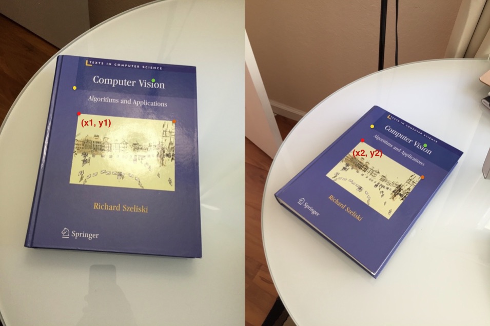
Consider two images of a plane (top of the book) shown in Figure 1. The red dot represents the same physical point in the two images. In computer vision jargon we call these corresponding points. Figure 1. shows four corresponding points in four different colors — red, green, yellow and orange. A Homography is a transformation ( a 3×3 matrix ) that maps the points in one image to the corresponding points in the other image.
Now since a homography is a 3×3 matrix we can write it as
![H = \left[ \begin {array} {ccc} h_{00} & h_{01} & h_{02} \\ h_{10} & h_{11} & h_{12} \\ h_{20} & h_{21} & h_{22} \end{array} \right]](https://learnopencv.com/wp-content/ql-cache/quicklatex.com-39c024dba489da8900f1b7adf918fca5_l3.png)
Let us consider the first set of corresponding points — ![]() in the first image and
in the first image and ![]() in the second image. Then, the Homography
in the second image. Then, the Homography ![]() maps them in the following way
maps them in the following way
![\left[ \begin{array}{c} x_1 \\ y_1 \\ 1 \end{array} \right]&= H \left[ \begin{array}{c} x_2 \\ y_2 \\ 1 \end{array} \right]&= \left[ \begin{array}{ccc} h_{00} & h_{01} & h_{02} \\ h_{10} & h_{11} & h_{12} \\ h_{20} & h_{21} & h_{22} \end{array} \right] \left[ \begin{array}{c}x_2 \\ y_2 \\1 \end{array} \right]](https://learnopencv.com/wp-content/ql-cache/quicklatex.com-f3524d81bb8e73f2dc24afbad99fc374_l3.png)
Homography examples using OpenCV – Image Alignment
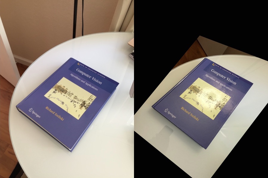
The above equation is true for ALL sets of corresponding points as long as they lie on the same plane in the real world. In other words you can apply the homography to the first image and the book in the first image will get aligned with the book in the second image! See Figure 2.

But what about points that are not on the plane ? Well, they will NOT be aligned by a homography as you can see in Figure 2. But wait, what if there are two planes in the image ? Well, then you have two homographies — one for each plane.
Homography examples using OpenCV – Panorama
In the previous section, we learned that if a homography between two images is known, we can warp one image onto the other. However, there was one big caveat. The images had to contain a plane ( the top of a book ), and only the planar part was aligned properly. It turns out that if you take a picture of any scene ( not just a plane ) and then take a second picture by rotating the camera, the two images are related by a homography!
In other words you can mount your camera on a tripod and take a picture. Next, pan it about the vertical axis and take another picture. The two images you just took of a completely arbitrary 3D scene are related by a homography. The two images will share some common regions that can be aligned and stitched and bingo you have a panorama of two images. Is it really that easy ? Nope! (sorry to disappoint) A lot more goes into creating a good panorama, but the basic principle is to align using a homography and stitch intelligently so that you do not see the seams. Creating panoramas will definitely be part of a future post.
How to calculate a Homography ?
To calculate a homography between two images, you need to know at least 4 point correspondences between the two images. If you have more than 4 corresponding points, it is even better. OpenCV will robustly estimate a homography that best fits all corresponding points. Usually, these point correspondences are found automatically by matching features like SIFT or SURF between the images, but in this post we are simply going to click the points by hand.
Let’s look at the usage first.
C++
// pts_src and pts_dst are vectors of points in source
// and destination images. They are of type vector<Point2f>.
// We need at least 4 corresponding points.

Mat h = findHomography(pts_src, pts_dst);

// The calculated homography can be used to warp
// the source image to destination. im_src and im_dst are
// of type Mat. Size is the size (width,height) of im_dst.
warpPerspective(im_src, im_dst, h, size);
Python
'''
pts_src and pts_dst are numpy arrays of points
in source and destination images. We need at least
4 corresponding points.
'''
h, status = cv2.findHomography(pts_src, pts_dst)

'''
The calculated homography can be used to warp
the source image to destination. Size is the
size (width,height) of im_dst
'''

im_dst = cv2.warpPerspective(im_src, h, size)
Let us look at a more complete example in both C++ and Python.
Homography examples using OpenCV C++
Images in Figure 2. can be generated using the following C++ code. The code below shows how to take four corresponding points in two images and warp image onto the other.
#include "opencv2/opencv.hpp"

using namespace cv;
using namespace std;

int main( int argc, char** argv)
{
    // Read source image.
    Mat im_src = imread("book2.jpg");
    // Four corners of the book in source image
    vector<Point2f> pts_src;
    pts_src.push_back(Point2f(141, 131));
    pts_src.push_back(Point2f(480, 159));
    pts_src.push_back(Point2f(493, 630));
    pts_src.push_back(Point2f(64, 601));

    // Read destination image.
    Mat im_dst = imread("book1.jpg");
    // Four corners of the book in destination image.
    vector<Point2f> pts_dst;
    pts_dst.push_back(Point2f(318, 256));
    pts_dst.push_back(Point2f(534, 372));
    pts_dst.push_back(Point2f(316, 670));
    pts_dst.push_back(Point2f(73, 473));

    // Calculate Homography
    Mat h = findHomography(pts_src, pts_dst);

    // Output image
    Mat im_out;
    // Warp source image to destination based on homography
    warpPerspective(im_src, im_out, h, im_dst.size());

    // Display images
    imshow("Source Image", im_src);
    imshow("Destination Image", im_dst);
    imshow("Warped Source Image", im_out);

    waitKey(0);
}
Homography examples using OpenCV Python
Images in Figure 2. can also be generated using the following Python code. The code below shows how to take four corresponding points in two images and warp image onto the other.
#!/usr/bin/env python

import cv2
import numpy as np

if __name__ == '__main__' :

    # Read source image.
    im_src = cv2.imread('book2.jpg')
    # Four corners of the book in source image
    pts_src = np.array([[141, 131], [480, 159], [493, 630],[64, 601]])

    # Read destination image.
    im_dst = cv2.imread('book1.jpg')
    # Four corners of the book in destination image.
    pts_dst = np.array([[318, 256],[534, 372],[316, 670],[73, 473]])

    # Calculate Homography
    h, status = cv2.findHomography(pts_src, pts_dst)

    # Warp source image to destination based on homography
    im_out = cv2.warpPerspective(im_src, h, (im_dst.shape[1],im_dst.shape[0]))

    # Display images
    cv2.imshow("Source Image", im_src)
    cv2.imshow("Destination Image", im_dst)
    cv2.imshow("Warped Source Image", im_out)

    cv2.waitKey(0)
Applications of Homography
The most interesting application of Homography is undoubtedly making panoramas ( a.k.a image mosaicing and image stitching ). Panoramas will be the subject of a later post. Let us see some other interesting applications.
Perspective Correction using Homography
Let’s say you have a photo shown in Figure 1. Wouldn’t it be cool if you could click on the four corners of the book and quickly get an image that looks like the one shown in Figure 3. You can get the code for this example in the download section below. Here are the steps.
- Write a user interface to collect four corners of the book. Let’s call these points pts_src
- We need to know the aspect ratio of the book. For this book, the aspect ratio ( width / height ) is 3/4. So we can choose the output image size to be 300×400, and our destination points ( pts_dst ) to be (0,0), (299,0), (299,399) and (0,399)
- Obtain the homography using pts_src and pts_dst .
- Apply the homography to the source image to obtain the image in Figure 3.
Virtual Billboard
In many televised sports events, advertisement in virtually inserted in live video feed. E.g. in soccer and baseball the ads placed on small advertisement boards right outside the boundary of the field can be virtually changed. Instead of displaying the same ad to everybody, advertisers can choose which ads to show based on the person’s demographics, location etc.
In these applications the four corners of the advertisement board are detected in the video which serve as the destination points. The four corners of the ad serve as the source points. A homography is calculated based on these four corresponding points and it is used to warp the ad into the video frame.
After reading this post you probably have an idea on how to put an image on a virtual billboard. Figure 4. shows the first image uploaded to the internet.
And Figure 5. shows The Times Square.

We can replace one of the billboards on The Times Square with the image of our choice. Here are the steps.
- Write a user interface to collect the four corners of the billboard in the image. Let’s call these points pts_dst
- Let the size of the image you want to put on the virtual billboard be w x h. The corners of the image ( pts_src ) are therefore to be (0,0), (w-1,0), (w-1,h-1) and (0,h-1)
- Obtain the homography using pts_src and pts_dst .
- Apply the homography to the source image and blend it with the destination image to obtain the image in Figure 6.
Notice in Figure 6. we have inserted image shown in Figure 4. into The Times Square Image.

Image Credits
- The image in Figure 4. was the first photographic image uploaded to the internet. It qualifies as fair use. [ link ]
- The image used in Figure 5. ( The Time Square ) is licensed under the GFDL. [ link ]


