Handwritten text documents are ubiquitous in the field of research and study. They are personalized to the user’s needs and often contain a style of writing difficult to comprehend by others. This becomes an issue for websites that deal with handwritten study notes. Several users upload their study material for collaboration, however, it can be difficult to understand the text.
Manually digitizing the notes requires effort on both fronts, understanding the text and typing it out. How can we solve this problem? This is where advanced OCR (Optical Character Recognition) models like TrOCR can help. In this article, we will carry out handwritten text recognition using OCR by fine-tuning the TrOCR model.
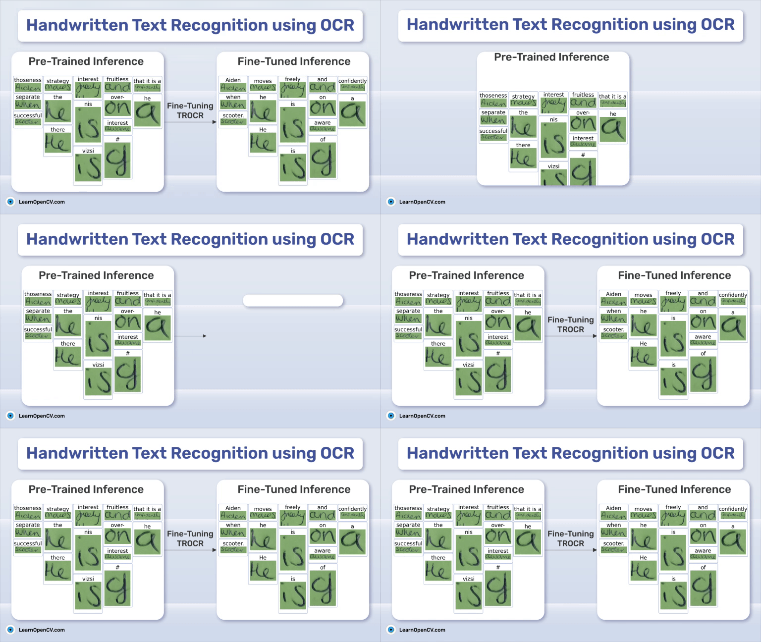
Our primary goal is to train a fast and performant OCR model that can recognize words in handwritten notes. Such fine-tuned models can help accelerate the process of digitizing notes which in turn can help in faster distribution to users.
However, training such models requires several steps spanning over data collection, preprocessing, fine-tuning, and evaluation.
We will focus on the following in this article:
- Discussing the GNHK dataset for handwritten notes recognition
- Preprocessing the dataset to make it training compliant
- Training the TrOCR model
- Running inference experiment to measure the performance qualitatively
Table of Contents
The GNHK Handwritten Notes Dataset
The GNHK (GoodNotes Handwriting Kollection) handwritten notes dataset by Goodnotes contains several hundred English handwritten notes by students worldwide.
The primary aim of this dataset is to encourage researchers and developers to investigate new methods of text recognition and localization for handwritten text in the wild.
We can download the text by scrolling to the bottom of the page, agreeing to the terms and conditions, and clicking the second link.
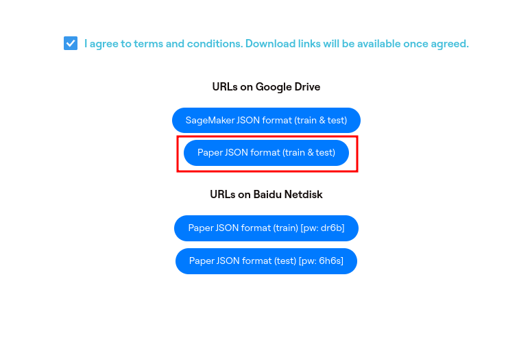
It will download the train_data.zip and test_data.zip files.
Extracting them will reveal the following structure.
├── test_data
│   └── test
│       ├── eng_AF_004.jpg
│       ├── eng_AF_004.json
│       ├── eng_AF_007.jpg
│       ├── eng_AF_007.json
│       ...
│       ├── eng_NA_142.jpg
│       └── eng_NA_142.json
├── train_data
    └── train
        ├── eng_AF_001.jpg
        ├── eng_AF_001.json
        ├── eng_AF_002.jpg
        ├── eng_AF_002.json
        ...
        ├── eng_NA_146.jpg
        └── eng_NA_146.json
4 directories, 1375 files
Each directory has a JPG image file and a corresponding JSON annotation file. There are 515 training samples and 172 validation samples. The images are high resolution, ranging from 1080p to 4K.
Following are a few of the image samples from the dataset.
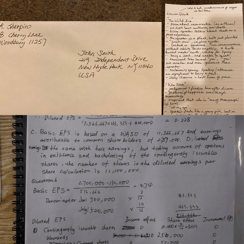
As we can see, most of the notes are extremely difficult to comprehend. Such personalized notes cannot be used by others easily.
Each image is accompanied by a single JSON file with contents in the following format (truncated for brevity).
[{"text": "%math%", "polygon": {"x0": 112, "y0": 556, "x1": 285, "y1": 563, "x2": 245, "y2": 776, "x3": 112, "y3": 783}, "line_idx": 1, "type": "H"}, {"text": "%math%", "polygon": {"x0": 2365, "y0": 202, "x1": 2350, "y1": 509, "x2": 2588, "y2": 527, "x3": 2632, "y3": 195}, "line_idx": 0, "type": "H"}, ... {"text": "ownership", "polygon": {"x0": 1347, "y0": 1606, "x1": 2238, "y1": 1574, "x2": 2170, "y2": 1884, "x3": 1300, "y3": 1747}, "line_idx": 4, "type": "H"}]
Each word contains its information in a dictionary with annotations of different words separated by a comma.
The first key is "text". If the word is either a mathematical symbol, a special character, or something that is not comprehensible, e.g., a strikethrough, then it is represented by a special word within the %% symbol. Otherwise, the "text" key contains the value as the actual word in the document.
The second important key that we need to focus on is the "polygon" key. This gives a multipoint polygon coordinate for each word. As we will see in the next section, this is important for the processing of the dataset.
The Directory Structure
Before moving further, let’s take a look at the entire project directory structure.
├── input
│   └── gnhk_dataset
│       ├── test_data
│       ├── test_processed
│       ├── train_data
│       ├── train_processed
│       ├── test_processed.csv
│       └── train_processed.csv
├── pretrained_model_inference  [10066 entries exceeds filelimit, not opening dir]
├── trocr_handwritten
│   ├── checkpoint-6093
│   │   ├── config.json
│   │   ├── generation_config.json
│   │   ├── model.safetensors
│   │   ├── optimizer.pt
│   │   ├── preprocessor_config.json
│   │   ├── rng_state.pth
│   │   ├── scheduler.pt
│   │   ├── trainer_state.json
│   │   └── training_args.bin
│   ├── checkpoint-6770
│   │   ├── config.json
│   │   ├── generation_config.json
│   │   ├── model.safetensors
│   │   ├── optimizer.pt
│   │   ├── preprocessor_config.json
│   │   ├── rng_state.pth
│   │   ├── scheduler.pt
│   │   ├── trainer_state.json
│   │   └── training_args.bin
│   └── runs
│       └── Aug27_11-30-05_f57a2dab37c7
├── Fine_Tune_TrOCR_Handwritten.ipynb
├── preprocess_gnhk_dataset.py
└── Pretrained_Model_Inference.ipynb
- The
input/gnhk_datasetcontains the dataset that we initially downloaded and extracted. - The
pretrained_model_inferencedirectory contains the inference results from the validation dataset using the pretrained TrOCR handwritten model. We will analyze these results in one of the later sections. - In the
trocr_handwrittendirectory we have the results after fine-tuning the TrOCR model. - We have two Jupyter Notebooks, one for fine tuning the model, and the other for running inference using the pretrained model.
- Finally, the
preprocess_gnhk_dataset.pyPython file contains the code for preprocessing the GNHK dataset.
Installing the Dependencies
We need to install the following dependencies before moving forward. This is necessary for preprocessing the dataset, inference, and training.
pip install transformers
pip install sentencepiece
pip install jiwer
pip install datasets
pip install evaluate
pip install -U accelerate
pip install matplotlib
pip install protobuf==3.20.1
pip install tensorboard
To know more about some of the major dependencies, you can go through the TrOCR fine tuning article where we train the model to recognize curved text in the wild.
Preprocessing the GNHK Dataset
The pretrained TrOCR model can only OCR single words or single-line sentences. However, the GNHK dataset contains images of entire documents. So, we cannot just feed these to the TrOCR model and expect it to perform well.
To tackle this problem and also prepare the final training dataset, we will take the help of the JSON files that come with the dataset.
We will employ the following steps to preprocess the dataset:
- Each JSON file contains the polygon coordinates for each word. We will convert these polygon coordinates to four-point bounding box coordinates first.
- Then, we will crop each word inside the bounding box and store them in a separate directory.
- We will also create two CSV files, one for the training set and one for the test set. They will contain the cropped image names and the label text.
Following is the code from the preprocess_gnhk_dataset.py file that processes the original dataset.
import os
import json
import csv
import cv2
import numpy as np
from tqdm import tqdm

def create_directories():
   dirs = [
       'input/gnhk_dataset/train_processed/images',
       'input/gnhk_dataset/test_processed/images',
   ]
   for dir_path in dirs:
       os.makedirs(dir_path, exist_ok=True)

def polygon_to_bbox(polygon):
   points = np.array([(polygon[f'x{i}'], polygon[f'y{i}']) for i in range(4)], dtype=np.int32)
   x, y, w, h = cv2.boundingRect(points)
   return x, y, w, h

def process_dataset(input_folder, output_folder, csv_path):
   with open(csv_path, 'w', newline='') as csvfile:
       csv_writer = csv.writer(csvfile)
       csv_writer.writerow(['image_filename', 'text'])

       for filename in tqdm(os.listdir(input_folder), desc=f"Processing {os.path.basename(input_folder)}"):
           if filename.endswith('.json'):
               json_path = os.path.join(input_folder, filename)
               img_path = os.path.join(input_folder, filename.replace('.json', '.jpg'))

               with open(json_path, 'r') as f:
                   data = json.load(f)

               img = cv2.imread(img_path)

               for idx, item in enumerate(data):
                   text = item['text']
                   if text.startswith('%') and text.endswith('%'):
                       text = 'SPECIAL_CHARACTER'

                   x, y, w, h = polygon_to_bbox(item['polygon'])

                   cropped_img = img[y:y+h, x:x+w]

                   output_filename = f"{filename.replace('.json', '')}_{idx}.jpg"
                   output_path = os.path.join(output_folder, output_filename)
                   cv2.imwrite(output_path, cropped_img)

                   csv_writer.writerow([output_filename, text])

def main():
   create_directories()

   process_dataset(
       'input/gnhk_dataset/train_data/train',
       'input/gnhk_dataset/train_processed/images',
       'input/gnhk_dataset/train_processed.csv'
   )
   process_dataset(
       'input/gnhk_dataset/test_data/test',
       'input/gnhk_dataset/test_processed/images',
       'input/gnhk_dataset/test_processed.csv'
   )

if __name__ == '__main__':
   main()
We can run the script with the following command.
$ python preprocess_gnhk_dataset.py
This will create two subdirectories in input/gnhk_dataset; train_processed/images and test_processed/images. Along with that, it will also generate the train_processed.csv and test_processed.csv files.
The following are some of the cropped images after processing.
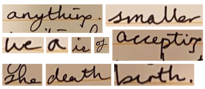
And this is what the CSV files look like.
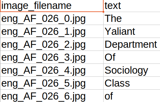
Each CSV file contains the cropped image name and the associated text label.
The final processed dataset contains 32,495 cropped training images and 10,066 cropped test images.
Analyzing Results From the Pretrained TrOCR Model
As Hugging Face provides TrOCR models pretrained on the handwritten dataset, we can do a baseline analysis on the test dataset. The Pretrained_Model_Inference.ipynb notebook contains the code that carries out the process. The notebook uses the microsoft/trocr-small-handwritten model for this inference step.
Running the notebook stores the result in the pretrained_model_inference directory.
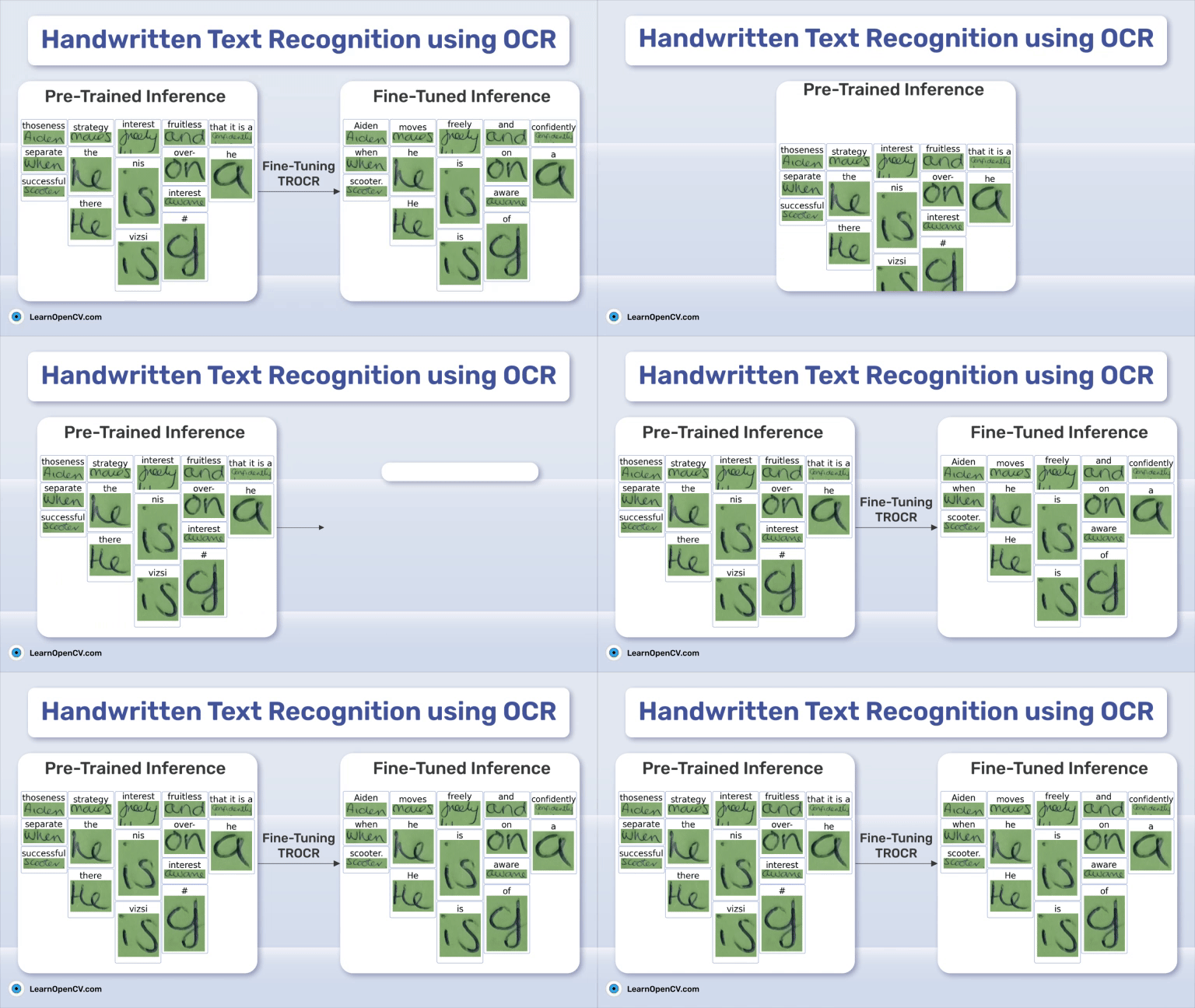
Here are a few cropped texts along with their inference for a sentence in one of the documents.

As we can see, almost all the OCR’d text is wrong. Fine tuning the model further on the training set would surely help to obtain better results.
Fine Tuning TrOCR for Handwritten Text Recognition
Now, let’s jump into the code for fine tuning the TrOCR Small Handwritten model.
The code that we will discuss here is present in the Fine_Tune_TrOCR_Handwritten.ipynb notebook.
Let’s start with the imports and define the necessary global settings.
import os
import torch
import evaluate
import numpy as np
import pandas as pd
import glob as glob
import torch.optim as optim
import matplotlib.pyplot as plt
import torchvision.transforms as transforms

from PIL import Image
from tqdm.notebook import tqdm
from dataclasses import dataclass
from torch.utils.data import Dataset
from transformers import (
   VisionEncoderDecoderModel,
   TrOCRProcessor,
   Seq2SeqTrainer,
   Seq2SeqTrainingArguments,
   default_data_collator
)

block_plot = False
plt.rcParams['figure.figsize'] = (12, 9)

os.environ["TOKENIZERS_PARALLELISM"] = 'false'
Next, we set the seed for reproducibility and initialize the computation device.
def seed_everything(seed_value):
   np.random.seed(seed_value)
   torch.manual_seed(seed_value)
   torch.cuda.manual_seed_all(seed_value)
   torch.backends.cudnn.deterministic = True
   torch.backends.cudnn.benchmark = False

seed_everything(42)

device = torch.device('cuda' if torch.cuda.is_available() else 'cpu')
Training and Dataset Configurations for Handwritten Text Recognition
We will use some important configurations throughout the notebook for training and dataset paths. The following code block initializes them.
@dataclass(frozen=True)
class TrainingConfig:
   BATCH_SIZE:    int = 48
   EPOCHS:        int = 10
   LEARNING_RATE: float = 0.00005

@dataclass(frozen=True)
class DatasetConfig:
   DATA_ROOT:     str = 'input/gnhk_dataset'

@dataclass(frozen=True)
class ModelConfig:
   MODEL_NAME: str = 'microsoft/trocr-small-handwritten'
We are using a batch size of 48 and will be training for 10 epochs with a base learning rate of 0.00005.
Furthermore, we also define the root dataset path and define the Hugging Face TrOCR model tag.
Visualizing the Cropped Sample with Labels
It’s always a good idea to visualize the sample before moving forward with the training. This gives us a validation that all the paths, CSV file preparation, and labeling were done correctly while preprocessing the dataset.
def visualize(dataset_path, df):
   all_images = df.image_filename
   all_labels = df.text

   plt.figure(figsize=(15, 3))
   for i in range(15):
       plt.subplot(3, 5, i+1)
       image = plt.imread(f"{dataset_path}/test_processed/images/{all_images[i]}")
       label = all_labels[i]
       plt.imshow(image)
       plt.axis('off')
       plt.title(label)
   plt.show()
sample_df = pd.read_csv(
   os.path.join(DatasetConfig.DATA_ROOT, 'test_processed.csv'),
   header=None,
   skiprows=1,
   names=['image_filename', 'text'],
   nrows=50
)

visualize(DatasetConfig.DATA_ROOT, sample_df)
We check the cropped images and the corresponding labels from one sentence in the test set.

GNHK Dataset Preparation
As the GNHK handwritten text recognition dataset has a custom directory structure and CSV files, we need to write the custom dataset preparation code as well.
Let’s start with reading the CSV files.
train_df = pd.read_csv(
   os.path.join(DatasetConfig.DATA_ROOT, 'train_processed.csv'),
   header=None,
   skiprows=1,
   names=['image_filename', 'text']
)


test_df = pd.read_csv(
   os.path.join(DatasetConfig.DATA_ROOT, 'test_processed.csv'),
   header=None,
   skiprows=1,
   names=['image_filename', 'text']
)
To mitigate the rate of overfitting, we will apply minor augmentation, primarily color jitter and gaussian blurring.
# Augmentations.
train_transforms = transforms.Compose([
   transforms.ColorJitter(brightness=.5, hue=.3),
   transforms.GaussianBlur(kernel_size=(3, 3), sigma=(0.1, 5)),
])
Next, we need to create a custom PyTorch dataset class.
class CustomOCRDataset(Dataset):
   def __init__(self, root_dir, df, processor, max_target_length=128):
       self.root_dir = root_dir
       self.df = df
       self.processor = processor
       self.max_target_length = max_target_length


       self.df['text'] = self.df['text'].fillna('')


   def __len__(self):
       return len(self.df)


   def __getitem__(self, idx):
       # The image file name.
       file_name = self.df['image_filename'][idx]
       # The text (label).
       text = self.df['text'][idx]

       # Read the image, apply augmentations, and get the transformed pixels.
       image = Image.open(self.root_dir + file_name).convert('RGB')
       image = train_transforms(image)
       pixel_values = self.processor(image, return_tensors='pt').pixel_values
       # Pass the text through the tokenizer and get the labels,
       # i.e. tokenized labels.
       labels = self.processor.tokenizer(
           text,
           padding='max_length',
           max_length=self.max_target_length
       ).input_ids
       # We are using -100 as the padding token.
       labels = [label if label != self.processor.tokenizer.pad_token_id else -100 for label in labels]
       encoding = {"pixel_values": pixel_values.squeeze(), "labels": torch.tensor(labels)}
       return encoding
The class initialization accepts the root directory path, the CSV file, the TrOCR processor, and the max length for the label generation and padding.
The entire processing happens in the __getitem__ method. We read the image, convert it to RGB format, and get the processed pixel values by passing the image through the TrOCR processor. The tokenizer tokenizes the text labels and pads them to a length of 128 tokens.
The next code block initializes the processor and prepares the training and validation datasets.
processor = TrOCRProcessor.from_pretrained(ModelConfig.MODEL_NAME)
train_dataset = CustomOCRDataset(
   root_dir=os.path.join(DatasetConfig.DATA_ROOT, 'train_processed/images/'),
   df=train_df,
   processor=processor
)
valid_dataset = CustomOCRDataset(
   root_dir=os.path.join(DatasetConfig.DATA_ROOT, 'test_processed/images/'),
   df=test_df,
   processor=processor
)
Initializing and Configuring the Model
Loading a model with the Transformers library is quite straightforward. We simply need to provide the model tag to the from_pretrained method.
model = VisionEncoderDecoderModel.from_pretrained(ModelConfig.MODEL_NAME)
model.to(device)
print(model)
# Total parameters and trainable parameters.
total_params = sum(p.numel() for p in model.parameters())
print(f"{total_params:,} total parameters.")
total_trainable_params = sum(
   p.numel() for p in model.parameters() if p.requires_grad)
print(f"{total_trainable_params:,} training parameters.")
The TrOCR Small Handwritten model contains 61.5 million parameters.
Further, we also need to set a few manual configurations for the model to train properly.
# Set special tokens used for creating the decoder_input_ids from the labels.
model.config.decoder_start_token_id = processor.tokenizer.cls_token_id
model.config.pad_token_id = processor.tokenizer.pad_token_id
# Set Correct vocab size.
model.config.vocab_size = model.config.decoder.vocab_size
model.config.eos_token_id = processor.tokenizer.sep_token_id

model.config.max_length = 64
model.config.early_stopping = True
model.config.no_repeat_ngram_size = 3
model.config.length_penalty = 2.0
model.config.num_beams = 4
The above code block carries out the following steps:
- Define the decoder start token ID and the pad token ID.
- Define the vocabulary size for proper configuration of the tokenizer.
- The maximum length that the model will output, early stopping for training, the N-gram size, and the number of beams for beam search.
These parameters are not a one-stop solution for all datasets. Tweaking these may be necessary when the nature of labels and the dataset changes.
Next, we define the AdamW optimizer with the configured learning rate and weight decay.
optimizer = optim.AdamW(
   model.parameters(), lr=TrainingConfig.LEARNING_RATE, weight_decay=0.0005
)
Character Error Rate (CER) – Evaluation Metric
OCR models are most commonly evaluated using CER which stands for Character Error Rate. The following code block loads the CER metric from the evaluate library and defines the compute_cer method.
cer_metric = evaluate.load('cer')


def compute_cer(pred):
   labels_ids = pred.label_ids
   pred_ids = pred.predictions


   pred_str = processor.batch_decode(pred_ids, skip_special_tokens=True)
   labels_ids[labels_ids == -100] = processor.tokenizer.pad_token_id
   label_str = processor.batch_decode(labels_ids, skip_special_tokens=True)


   cer = cer_metric.compute(predictions=pred_str, references=label_str)


   return {"cer": cer}
During evaluation, the padding tokens are converted to -100 to avoid influence over the metric value.
Training and Validation for Handwritten Text Recognition using OCR
Before we can begin the training, the training arguments and Trainer API need to be initialized.
training_args = Seq2SeqTrainingArguments(
   predict_with_generate=True,
   evaluation_strategy='epoch',
   per_device_train_batch_size=TrainingConfig.BATCH_SIZE,
   per_device_eval_batch_size=TrainingConfig.BATCH_SIZE,
   fp16=True,
   output_dir='trocr_handwritten/',
   logging_strategy='epoch',
   save_strategy='epoch',
   save_total_limit=2,
   report_to='tensorboard',
   num_train_epochs=TrainingConfig.EPOCHS,
   dataloader_num_workers=8
)
We have set the evaluation strategy to epochs so that the CER value is calculated on the validation set after each epoch. All the results will be stored in the trocr_handwritten directory. The loss and CER graphs will be logged to Tensorboard.
# Initialize trainer.
trainer = Seq2SeqTrainer(
   model=model,
   tokenizer=processor.feature_extractor,
   args=training_args,
   compute_metrics=compute_cer,
   train_dataset=train_dataset,
   eval_dataset=valid_dataset,
   data_collator=default_data_collator
)
The Seq2SeqTrainer API accepts the model, the processor, the training arguments defined above, the datasets, and the data collator as the arguments.
Finally, we need to call the train method of the Trainer API to start the fine-tuning process.
Following are logs after 10 epochs.
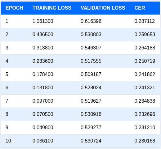
We get the best validation CER value after the last epoch. In the next section, we will use that checkpoint for running inference on the validation set.
The Tensorboard log gives more insight into the validation CER trend throughout the training.

The validation CER graph was going down till the end of training. With proper scheduling of the learning rate, we could train it for a few more epochs.
Inference using the Trained TrOCR Model
Moving forward, we will run inference on the same set of images we visualized in the initial sections of the article. We also have their inference results from the pretrained model. This makes it easy to compare the results.
Let’s load the processor and the trained checkpoint weights.
processor = TrOCRProcessor.from_pretrained(ModelConfig.MODEL_NAME)
trained_model = VisionEncoderDecoderModel.from_pretrained('trocr_handwritten/checkpoint-'+str(res.global_step)).to(device)
A few helper functions need to be defined for reading the images, forward passing through the model, and plotting.
def read_and_show(image_path):
   """
   :param image_path: String, path to the input image.


   Returns:
       image: PIL Image.
   """
   image = Image.open(image_path).convert('RGB')
   return image

def ocr(image, processor, model):
   """
   :param image: PIL Image.
   :param processor: Huggingface OCR processor.
   :param model: Huggingface OCR model.


   Returns:
       generated_text: the OCR'd text string.
   """
   pixel_values = processor(image, return_tensors='pt').pixel_values.to(device)
   generated_ids = model.generate(pixel_values)
   generated_text = processor.batch_decode(generated_ids, skip_special_tokens=True)[0]
   return generated_text

def eval_new_data(
   data_path=None,
   num_samples=50,
   df=None
):
   all_images = df.image_filename
   all_labels = df.text

   plt.figure(figsize=(15, 3))
   for i in range(num_samples):
       plt.subplot(3, 5, i+1)
       image = read_and_show(os.path.join(data_path, all_images[i]))
       text = ocr(image, processor, trained_model)
       plt.imshow(image)
       plt.title(text)
       plt.axis('off')
   plt.show()
Finally, provide the path to the evaluation set and visualize the first 15 results.
eval_new_data(
   data_path=os.path.join(DatasetConfig.DATA_ROOT, 'test_processed/images'),
   num_samples=15,
   df=sample_df
)
The results shown below are inferred from the TrOCR model trained on the handwritten text dataset.

Interestingly, the model predicted all the words correctly. This validates our entire process of fine tuning the handwritten text dataset.
Further Improvements
Above, we have implemented only part of the process for creating an OCR pipeline to digitize handwritten documents.
We can make the process more robust with the following steps:
- OCR on each word in the document is not ideal. It is much better to OCR each sentence. For this, we need to train a robust sentence detector model, like YOLOv10. This will make the management of the layout of the digitized document much easier.
- We can also train an OCR model which can detect different languages and translate them back to a target language.
- At the moment, our model does not handle mathematical and scientific symbols. Adding this feature will provide a better user experience.
Summary and Conclusions
In this article, we trained an OCR model for handwritten text recognition. We started with a real-world problem statement, discussed the dataset, the TrOCR model, and moved towards a simple POC.
After analyzing the results from the trained models, we also discussed some of the potential pitfalls and improvements of the current pipeline. You can take up any of these improvements as a challenge to implement. Let us know in the comments what you discover and build by expanding this project.



100K+ Learners
Join Free OpenCV Bootcamp3 Hours of Learning