


If you have been working with OpenCV for some time, you should have noticed that in most scenarios OpenCV utilizes CPU, which doesn’t always guarantee you the desired performance. To tackle this problem, in 2010 a new module that provides GPU acceleration using CUDA was added to OpenCV. You can find a benchmark demonstrating the advantage of the GPU module below:
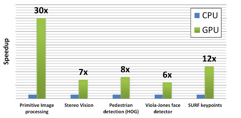
To find out the benchmark details, you can refer to the Realtime Computer Vision with OpenCV article.
Overview
Let’s briefly list what we will do in this post:
- Overview OpenCV modules that already have support for CUDA.
- Take a look at the basic block
cv::gpu::GpuMat(cv2.cuda_GpuMat). - Learn how to transfer data between CPU and GPU.
- Learn how to utilize multiple GPUs.
- Write a simple demo (both C++ and Python) to get to know the CUDA support API provided by OpenCV and to calculate the performance boost we can gain.
Supported Modules
Even though not all the library’s functionality is covered, it is claimed, that
the module “still keeps growing and is being adapted for the new computing technologies and GPU architectures.”
Let’s take a look at the official documentation of the CUDA-accelerated OpenCV. Here we can see listed modules that are already supported:
- Core part
- Operations on Matrices
- Background Segmentation
- Video Encoding/Decoding
- Feature Detection and Description
- Image Filtering
- Image Processing
- Legacy support
- Object Detection
- Optical Flow
- Stereo Correspondence
- Image Warping
- Device layer


Basic Block – GpuMat
To keep data in GPU memory, OpenCV introduces a new class cv::gpu::GpuMat (or cv2.cuda_GpuMat in Python) which serves as a primary data container. Its interface is similar to cv::Mat (cv2.Mat) making the transition to the GPU module as smooth as possible. Another thing worth mentioning is that all GPU functions receive GpuMat as input and output arguments. You can reduce the overhead on copying the data between the CPU and GPU with such design having chained GPU algorithms in your code.
CPU/GPU Data Transfer
To transfer data from GpuMat to Mat and vice-versa, OpenCV provides two functions:
- upload, which copies data from host memory to device memory
- download, which copies data from device memory to host memory.
Below is a simple example in C++ of their usage in a context:
#include <opencv2/highgui.hpp>
#include <opencv2/cudaimgproc.hpp>

cv::Mat img = cv::imread("image.png", IMREAD_GRAYSCALE);
cv::cuda::GpuMat dst, src;
src.upload(img);

cv::Ptr<cv::cuda::CLAHE> ptr_clahe = cv::cuda::createCLAHE(5.0, cv::Size(8, 8));
ptr_clahe->apply(src, dst);

cv::Mat result;
dst.download(result);

cv::imshow("result", result);
cv::waitKey();

And the same example in Python:
img = cv2.imread("image.png", cv2.IMREAD_GRAYSCALE)
src = cv2.cuda_GpuMat()
src.upload(img)

clahe = cv2.cuda.createCLAHE(clipLimit=5.0, tileGridSize=(8, 8))
dst = clahe.apply(src, cv2.cuda_Stream.Null())

result = dst.download()

cv2.imshow("result", result)
cv2.waitKey(0)
Utilizing Multiple GPUs
By default, each of the OpenCV CUDA algorithms uses a single GPU. If you need to utilize multiple GPUs, you have to manually distribute the work between GPUs. To switch active device use cv::cuda::setDevice (cv2.cuda.SetDevice) function.
Sample Demo
OpenCV provides samples on how to work with already implemented methods with GPU support using C++ API. But not so much information comes up when you want to try out Python API, which is also supported. Let’s implement a simple demo on how to use CUDA-accelerated OpenCV with C++ and Python API on the example of dense optical flow calculation using Farneback’s algorithm.
We will first take a look at how this could be done using the CPU. Then we will do the same using GPU. And finally, we are going to compare the elapsed time to calculate the gained speedup. Check out the README.md file with proper installation instructions before you start if you’d like to run the code yourself.
FPS Calculation
Since our primary goal is to find out how fast the algorithm works on different devices, we need to choose how we can measure it. A common way of doing so in the Computer Vision field is to calculate the number of processed frames per second (FPS). You can take a look at our earlier post for a quick reminder of how it could be done.
CPU Pipeline
1. Video and Its Attributes
We will start with video capture initialization and getting its attributes such as frame rate and a number of its frames. This part is common for CPU and GPU part:
Python
    # init video capture with video
    cap = cv2.VideoCapture(video)

    # get default video FPS
    fps = cap.get(cv2.CAP_PROP_FPS)

    # get total number of video frames
    num_frames = cap.get(cv2.CAP_PROP_FRAME_COUNT)
C++
    // init video capture with video
    VideoCapture capture(videoFileName);
    if (!capture.isOpened())
    {
        // error in opening the video file
        cout << "Unable to open file!" << endl;
        return;
    }

    // get default video FPS
    double fps = capture.get(CAP_PROP_FPS);

    // get total number of video frames
    int num_frames = int(capture.get(CAP_PROP_FRAME_COUNT));
2. Reading the First Frame
Because of the specificity of the algorithm, that uses two frames for calculation, we need to read the first frame before we move on. Some pre-processing is also needed such as resizing and converting to grayscale:
Python
    # read the first frame
    ret, previous_frame = cap.read()

    if device == "cpu":

        # proceed if frame reading was successful
        if ret:
            # resize frame
            frame = cv2.resize(previous_frame, (960, 540))

            # convert to gray
            previous_frame = cv2.cvtColor(frame, cv2.COLOR_BGR2GRAY)

            # create hsv output for optical flow
            hsv = np.zeros_like(frame, np.float32)

            # set saturation to 1
            hsv[..., 1] = 1.0
C++
    // read the first frame
    cv::Mat frame, previous_frame;
    capture >> frame;

    if (device == "cpu")
    {
        // resize frame
        cv::resize(frame, frame, Size(960, 540), 0, 0, INTER_LINEAR);

        // convert to gray
        cv::cvtColor(frame, previous_frame, COLOR_BGR2GRAY);

        // declare outputs for optical flow
        cv::Mat magnitude, normalized_magnitude, angle;
        cv::Mat hsv[3], merged_hsv, hsv_8u, bgr;

        // set saturation to 1
        hsv[1] = cv::Mat::ones(frame.size(), CV_32F);
You may notice, that we’ve also created an output frame, which we will use later.
3. Reading and Pre-processing Other Frames
Before reading the rest frames in a loop, we start two timers: one will track the full pipeline working time, the second one – reading frame time. Since Farneback’s Optical Flow algorithm works with grayscale frames, we need to make sure, we’re passing a grayscale video as an input. That’s why we first pre-process it to convert each frame from BGR format to grayscale. Also, since the original resolution might be too large, we resize it to a smaller size the same way as we did it for the first frame. We set up one more timer to calculate the time spent on the pre-processing stage:
Python
                while True:
                # start full pipeline timer
                start_full_time = time.time()

                # start reading timer
                start_read_time = time.time()

                # capture frame-by-frame
                ret, frame = cap.read()

                # end reading timer
                end_read_time = time.time()

                # add elapsed iteration time
                timers["reading"].append(end_read_time - start_read_time)

                # if frame reading was not successful, break
                if not ret:
                    break

                # start pre-process timer
                start_pre_time = time.time()
                # resize frame
                frame = cv2.resize(frame, (960, 540))

                # convert to gray
                current_frame = cv2.cvtColor(frame, cv2.COLOR_BGR2GRAY)

                # end pre-process timer
                end_pre_time = time.time()

                # add elapsed iteration time
                timers["pre-process"].append(end_pre_time - start_pre_time)
C++
        while (true)
        {
            // start full pipeline timer
            auto start_full_time = high_resolution_clock::now();

            // start reading timer
            auto start_read_time = high_resolution_clock::now();

            // capture frame-by-frame
            capture >> frame;

            if (frame.empty())
                break;

            // end reading timer
            auto end_read_time = high_resolution_clock::now();

            // add elapsed iteration time
            timers["reading"].push_back(duration_cast<milliseconds>(end_read_time - start_read_time).count() / 1000.0);

            // start pre-process timer
            auto start_pre_time = high_resolution_clock::now();

            // resize frame
            cv::resize(frame, frame, Size(960, 540), 0, 0, INTER_LINEAR);

            // convert to gray
            cv::Mat current_frame;
            cv::cvtColor(frame, current_frame, COLOR_BGR2GRAY);

            // end pre-process timer
            auto end_pre_time = high_resolution_clock::now();

            // add elapsed iteration time
            timers["pre-process"].push_back(duration_cast<milliseconds>(end_pre_time - start_pre_time).count() / 1000.0);
4. Calculating Dense Optical Flow
We use the corresponding method called calcOpticalFlowFarneback to calculate a dense optical flow between two frames:
Python
                # start optical flow timer
                start_of = time.time()

                # calculate optical flow
                flow = cv2.calcOpticalFlowFarneback(
                    previous_frame, current_frame, None, 0.5, 5, 15, 3, 5, 1.2, 0,
                )
                # end of timer
                end_of = time.time()

                # add elapsed iteration time
                timers["optical flow"].append(end_of - start_of)
C++
            // start optical flow timer
            auto start_of_time = high_resolution_clock::now();

            // calculate optical flow
            cv::Mat flow;
            calcOpticalFlowFarneback(previous_frame, current_frame, flow, 0.5, 5, 15, 3, 5, 1.2, 0);

            // end optical flow timer
            auto end_of_time = high_resolution_clock::now();

            // add elapsed iteration time
            timers["optical flow"].push_back(duration_cast<milliseconds>(end_of_time - start_of_time).count() / 1000.0);
We wrap its usage in-between two timers calls, again, to calculate the elapsed time.
5. Post-processing
Farneback’s Optical Flow algorithm output a two-dimensional flow vector. We convert these outputs to polar coordinates to obtain the angle (direction) of flow by hue and the distance (magnitude) of flow by value of HSV color representation. For visualization, all we have left to do now is to convert the result to BGR space. After that we stop all the remained timers to get the elapsed time:
Python
                # start post-process timer
                start_post_time = time.time()

                # convert from cartesian to polar coordinates to get magnitude and angle
                magnitude, angle = cv2.cartToPolar(
                    flow[..., 0], flow[..., 1], angleInDegrees=True,
                )

                # set hue according to the angle of optical flow
                hsv[..., 0] = angle * ((1 / 360.0) * (180 / 255.0))

                # set value according to the normalized magnitude of optical flow
                hsv[..., 2] = cv2.normalize(
                    magnitude, None, 0.0, 1.0, cv2.NORM_MINMAX, -1,
                )

                # multiply each pixel value to 255
                hsv_8u = np.uint8(hsv * 255.0)

                # convert hsv to bgr
                bgr = cv2.cvtColor(hsv_8u, cv2.COLOR_HSV2BGR)

                # update previous_frame value
                previous_frame = current_frame

                # end post-process timer
                end_post_time = time.time()

                # add elapsed iteration time
                timers["post-process"].append(end_post_time - start_post_time)

                # end full pipeline timer
                end_full_time = time.time()

                # add elapsed iteration time
                timers["full pipeline"].append(end_full_time - start_full_time)
C++
            // start post-process timer
            auto start_post_time = high_resolution_clock::now();

            // split the output flow into 2 vectors
            cv::Mat flow_xy[2], flow_x, flow_y;
            split(flow, flow_xy);

            // get the result
            flow_x = flow_xy[0];
            flow_y = flow_xy[1];

            // convert from cartesian to polar coordinates
            cv::cartToPolar(flow_x, flow_y, magnitude, angle, true);

            // normalize magnitude from 0 to 1
            cv::normalize(magnitude, normalized_magnitude, 0.0, 1.0, NORM_MINMAX);

            // get angle of optical flow
            angle *= ((1 / 360.0) * (180 / 255.0));

            // build hsv image
            hsv[0] = angle;
            hsv[2] = normalized_magnitude;
            merge(hsv, 3, merged_hsv);

            // multiply each pixel value to 255
            merged_hsv.convertTo(hsv_8u, CV_8U, 255);

            // convert hsv to bgr
            cv::cvtColor(hsv_8u, bgr, COLOR_HSV2BGR);

            // update previous_frame value
            previous_frame = current_frame;

            // end post pipeline timer
            auto end_post_time = high_resolution_clock::now();

            // add elapsed iteration time
            timers["post-process"].push_back(duration_cast<milliseconds>(end_post_time - start_post_time).count() / 1000.0);

            // end full pipeline timer
            auto end_full_time = high_resolution_clock::now();

            // add elapsed iteration time
            timers["full pipeline"].push_back(duration_cast<milliseconds>(end_full_time - start_full_time).count() / 1000.0);
6. Visualization
We visualize the original frame resized to 960×540 and the result using imshow function:
Python
                # visualization
                cv2.imshow("original", frame)
                cv2.imshow("result", bgr)
                k = cv2.waitKey(1)
                if k == 27:
                    break
C++
            // visualization
            imshow("original", frame);
            imshow("result", bgr);
            int keyboard = waitKey(1);
            if (keyboard == 27)
                break;
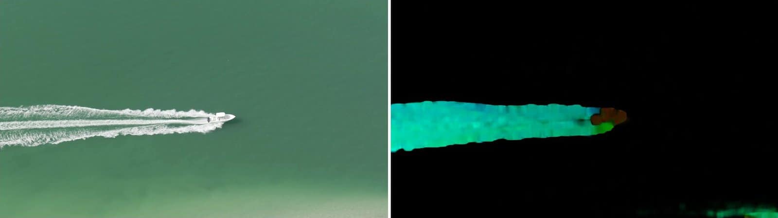
Here’s what we get with a sample “boat.mp4” video:
7. Time and FPS Calculation
All we have to do is to calculate the elapsed time at each step of the pipeline and measure FPS for optical flow part and the full pipeline:
Python
    # elapsed time at each stage
    print("Elapsed time")
    for stage, seconds in timers.items():
        print("-", stage, ": {:0.3f} seconds".format(sum(seconds)))

    # calculate frames per second
    print("Default video FPS : {:0.3f}".format(fps))

    of_fps = (num_frames - 1) / sum(timers["optical flow"])
    print("Optical flow FPS : {:0.3f}".format(of_fps))

    full_fps = (num_frames - 1) / sum(timers["full pipeline"])
    print("Full pipeline FPS : {:0.3f}".format(full_fps))
C++
    // elapsed time at each stage
    cout << "Elapsed time" << std::endl;
    for (auto const& timer : timers)
    {
        cout << "- " << timer.first << " : " << accumulate(timer.second.begin(), timer.second.end(), 0.0) << " seconds"<< endl;
    }

    // calculate frames per second
    cout << "Default video FPS : "  << fps << endl;
    float optical_flow_fps  = (num_frames - 1) / accumulate(timers["optical flow"].begin(),  timers["optical flow"].end(),  0.0);
    cout << "Optical flow FPS : "   << optical_flow_fps  << endl;

    float full_pipeline_fps = (num_frames - 1) / accumulate(timers["full pipeline"].begin(), timers["full pipeline"].end(), 0.0);
    cout << "Full pipeline FPS : "  << full_pipeline_fps << endl;
GPU Pipeline
The algorithm stays the same with moving it to CUDA but has some differences connected to the GPU usage. Let’s go through the pipeline once again and see what has changed:
1. Video and Its Attributes
This part is common in both CPU and GPU part, so it stays the same.
2. Reading the First Frame
Notice, that we use the same CPU functions for reading and resizing, but upload the result to cv::cuda::GpuMat (cuda_GpuMat) instance:
Python
        # proceed if frame reading was successful
        if ret:
            # resize frame
            frame = cv2.resize(previous_frame, (960, 540))

            # upload resized frame to GPU
            gpu_frame = cv2.cuda_GpuMat()
            gpu_frame.upload(frame)

            # convert to gray
            previous_frame = cv2.cvtColor(frame, cv2.COLOR_BGR2GRAY)

            # upload pre-processed frame to GPU
            gpu_previous = cv2.cuda_GpuMat()
            gpu_previous.upload(previous_frame)

            # create gpu_hsv output for optical flow
            gpu_hsv = cv2.cuda_GpuMat(gpu_frame.size(), cv2.CV_32FC3)
            gpu_hsv_8u = cv2.cuda_GpuMat(gpu_frame.size(), cv2.CV_8UC3)

            gpu_h = cv2.cuda_GpuMat(gpu_frame.size(), cv2.CV_32FC1)
            gpu_s = cv2.cuda_GpuMat(gpu_frame.size(), cv2.CV_32FC1)
            gpu_v = cv2.cuda_GpuMat(gpu_frame.size(), cv2.CV_32FC1)

            # set saturation to 1
            gpu_s.upload(np.ones_like(previous_frame, np.float32))
C++
        // resize frame
        cv::resize(frame, frame, Size(960, 540), 0, 0, INTER_LINEAR);

        // convert to gray
        cv::cvtColor(frame, previous_frame, COLOR_BGR2GRAY);

        // upload pre-processed frame to GPU
        cv::cuda::GpuMat gpu_previous;
        gpu_previous.upload(previous_frame);

        // declare cpu outputs for optical flow
        cv::Mat hsv[3], angle, bgr;

        // declare gpu outputs for optical flow
        cv::cuda::GpuMat gpu_magnitude, gpu_normalized_magnitude, gpu_angle;
        cv::cuda::GpuMat gpu_hsv[3], gpu_merged_hsv, gpu_hsv_8u, gpu_bgr;

        // set saturation to 1
        hsv[1] = cv::Mat::ones(frame.size(), CV_32F);
        gpu_hsv[1].upload(hsv[1]);
3. Reading and Pre-processing Other Frames
Python
            while True:
                # start full pipeline timer
                start_full_time = time.time()

                # start reading timer
                start_read_time = time.time()

                # capture frame-by-frame
                ret, frame = cap.read()

                # upload frame to GPU
                gpu_frame.upload(frame)

                # end reading timer
                end_read_time = time.time()

                # add elapsed iteration time
                timers["reading"].append(end_read_time - start_read_time)

                # if frame reading was not successful, break
                if not ret:
                    break

                # start pre-process timer
                start_pre_time = time.time()

                # resize frame
                gpu_frame = cv2.cuda.resize(gpu_frame, (960, 540))

                # convert to gray
                gpu_current = cv2.cuda.cvtColor(gpu_frame, cv2.COLOR_BGR2GRAY)

                # end pre-process timer
                end_pre_time = time.time()
C++
        while (true)
        {
            // start full pipeline timer
            auto start_full_time = high_resolution_clock::now();

            // start reading timer
            auto start_read_time = high_resolution_clock::now();

            // capture frame-by-frame
            capture >> frame;

            if (frame.empty())
                break;

            // upload frame to GPU
            cv::cuda::GpuMat gpu_frame;
            gpu_frame.upload(frame);

            // end reading timer
            auto end_read_time = high_resolution_clock::now();

            // add elapsed iteration time
            timers["reading"].push_back(duration_cast<milliseconds>(end_read_time - start_read_time).count() / 1000.0);

            // start pre-process timer
            auto start_pre_time = high_resolution_clock::now();

            // resize frame
            cv::cuda::resize(gpu_frame, gpu_frame, Size(960, 540), 0, 0, INTER_LINEAR);

            // convert to gray
            cv::cuda::GpuMat gpu_current;
            cv::cuda::cvtColor(gpu_frame, gpu_current, COLOR_BGR2GRAY);

            // end pre-process timer
            auto end_pre_time = high_resolution_clock::now();

            // add elapsed iteration time
            timers["pre-process"].push_back(duration_cast<milliseconds>(end_pre_time - start_pre_time).count() / 1000.0);
4. Calculating Dense Optical Flow
Instead of using cv::calcOpticalFlowFarneback (cv2.calcOpticalFlowFarneback) function call, we first use cv::cuda::FarnebackOpticalFlow::create (cv2.cuda_FarnebackOpticalFlow.create) to create an instance of cuda_FarnebackOpticalFlow class and then call cv::cuda::FarnebackOpticalFlow::calc(cv2.cuda_FarnebackOpticalFlow.calc) to calculate optical flow between two frames:
Python
                # start optical flow timer
                start_of = time.time()

                # create optical flow instance
                gpu_flow = cv2.cuda_FarnebackOpticalFlow.create(
                    5, 0.5, False, 15, 3, 5, 1.2, 0,
                )
                # calculate optical flow
                gpu_flow = cv2.cuda_FarnebackOpticalFlow.calc(
                    gpu_flow, gpu_previous, gpu_current, None,
                )

                # end of timer
                end_of = time.time()

                # add elapsed iteration time
                timers["optical flow"].append(end_of - start_of)
C++
            // start optical flow timer
            auto start_of_time = high_resolution_clock::now();

            // create optical flow instance
            Ptr<cuda::FarnebackOpticalFlow> ptr_calc = cuda::FarnebackOpticalFlow::create(5, 0.5, false, 15, 3, 5, 1.2, 0);
            // calculate optical flow
            cv::cuda::GpuMat gpu_flow;
            ptr_calc->calc(gpu_previous, gpu_current, gpu_flow);

            // end optical flow timer
            auto end_of_time = high_resolution_clock::now();

            // add elapsed iteration time
            timers["optical flow"].push_back(duration_cast<milliseconds>(end_of_time - start_of_time).count() / 1000.0);
5. Post-processing
For post-processing, we use GPU variant of the same function as we used in CPU pipeline:
Python
                # start post-process timer
                start_post_time = time.time()

                gpu_flow_x = cv2.cuda_GpuMat(gpu_flow.size(), cv2.CV_32FC1)
                gpu_flow_y = cv2.cuda_GpuMat(gpu_flow.size(), cv2.CV_32FC1)
                cv2.cuda.split(gpu_flow, [gpu_flow_x, gpu_flow_y])

                # convert from cartesian to polar coordinates to get magnitude and angle
                gpu_magnitude, gpu_angle = cv2.cuda.cartToPolar(
                    gpu_flow_x, gpu_flow_y, angleInDegrees=True,
                )

                # set value to normalized magnitude from 0 to 1
                gpu_v = cv2.cuda.normalize(gpu_magnitude, 0.0, 1.0, cv2.NORM_MINMAX, -1)

                # get angle of optical flow
                angle = gpu_angle.download()
                angle *= (1 / 360.0) * (180 / 255.0)

                # set hue according to the angle of optical flow
                gpu_h.upload(angle)

                # merge h,s,v channels
                cv2.cuda.merge([gpu_h, gpu_s, gpu_v], gpu_hsv)

                # multiply each pixel value to 255
                gpu_hsv.convertTo(cv2.CV_8U, 255.0, gpu_hsv_8u, 0.0)

                # convert hsv to bgr
                gpu_bgr = cv2.cuda.cvtColor(gpu_hsv_8u, cv2.COLOR_HSV2BGR)

                # send original frame from GPU back to CPU
                frame = gpu_frame.download()

                # send result from GPU back to CPU
                bgr = gpu_bgr.download()

                # update previous_frame value
                gpu_previous = gpu_current

                # end post-process timer
                end_post_time = time.time()

                # add elapsed iteration time
                timers["post-process"].append(end_post_time - start_post_time)

                # end full pipeline timer
                end_full_time = time.time()

                # add elapsed iteration time
                timers["full pipeline"].append(end_full_time - start_full_time)
C++
            // start post-process timer
            auto start_post_time = high_resolution_clock::now();

            // split the output flow into 2 vectors
            cv::cuda::GpuMat gpu_flow_xy[2];
            cv::cuda::split(gpu_flow, gpu_flow_xy);

            // convert from cartesian to polar coordinates
            cv::cuda::cartToPolar(gpu_flow_xy[0], gpu_flow_xy[1], gpu_magnitude, gpu_angle, true);

            // normalize magnitude from 0 to 1
            cv::cuda::normalize(gpu_magnitude, gpu_normalized_magnitude, 0.0, 1.0, NORM_MINMAX, -1);

            // get angle of optical flow
            gpu_angle.download(angle);
            angle *= ((1 / 360.0) * (180 / 255.0));

            // build hsv image
            gpu_hsv[0].upload(angle);
            gpu_hsv[2] = gpu_normalized_magnitude;
            cv::cuda::merge(gpu_hsv, 3, gpu_merged_hsv);

            // multiply each pixel value to 255
            gpu_merged_hsv.cv::cuda::GpuMat::convertTo(gpu_hsv_8u, CV_8U, 255.0);

            // convert hsv to bgr
            cv::cuda::cvtColor(gpu_hsv_8u, gpu_bgr, COLOR_HSV2BGR);

            // send original frame from GPU back to CPU
            gpu_frame.download(frame);

            // send result from GPU back to CPU
            gpu_bgr.download(bgr);

            // update previous_frame value
            gpu_previous = gpu_current;

            // end post pipeline timer
            auto end_post_time = high_resolution_clock::now();

            // add elapsed iteration time
            timers["post-process"].push_back(duration_cast<milliseconds>(end_post_time - start_post_time).count() / 1000.0);

            // end full pipeline timer
            auto end_full_time = high_resolution_clock::now();

            // add elapsed iteration time
            timers["full pipeline"].push_back(duration_cast<milliseconds>(end_full_time - start_full_time).count() / 1000.0);
Also note, that we use download function to move the result back to CPU before visualization.
6. Visualization
The visualization part is common for CPU and GPU pipelines and stays the same.
7. Time and FPS Calculation
That stage also stays the same.
Results
Now we’re ready to compare metrics from CPU and GPU versions on a sample video. The configuration we use for CPU is:
Intel Core i7-8700
After running the script using a CPU device the result is:
Configuration
- device : cpu
- video file : video/boat.mp4
Number of frames: 320
Elapsed time
- full pipeline : 37.355 seconds
- reading : 3.327 seconds
- pre-process : 0.027 seconds
- optical flow : 32.706 seconds
- post-process : 0.641 seconds
Default video FPS : 29.97
Optical flow FPS : 9.75356
Full pipeline FPS : 8.53969
The configuration we use for GPU is:
Nvidia GeForce GTX 1080 Ti
And after running the script using a GPU device we get:
Configuration
- device : gpu
- video file : video/boat.mp4
Number of frames: 320
Elapsed time
- full pipeline : 8.665 seconds
- reading : 4.821 seconds
- pre-process : 0.035 seconds
- optical flow : 1.874 seconds
- post-process : 0.631 seconds
Default video FPS : 29.97
Optical flow FPS : 170.224
Full pipeline FPS : 36.8148
That gives us a ~17x speedup of the optical flow calculation when we use CUDA-acceleration! But unfortunately, we live in a real-word, where not all of the stages of the pipeline can be accelerated. Because of that, for the whole pipeline, we only got ~4 times speedup.
Conclusion
In our today’s post, we’ve overviewed the GPU OpenCV module and wrote a simple demo to find out how Farneback’s Optical Flow algorithm can be accelerated. We looked at API that OpenCV provides for this module, which you can reuse to try your hands at accelerating OpenCV algorithms with CUDA as well.