Generative and Discriminative Models

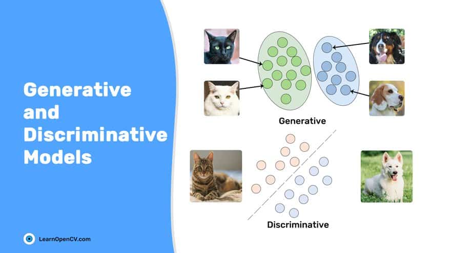
Most of the Machine Learning and Deep Learning problems that you solve are conceptualized from the Generative and Discriminative Models. In Machine Learning, one can clearly distinguish between the two modelling types:

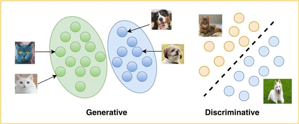
• Classifying an image as a dog or a cat falls under Discriminative Modelling
• Producing a realistic dog or a cat image is a Generative Modelling problem

The more the neural networks got adopted, the more the generative and discriminative domains grew. To understand the algorithms based on these models, you need to study the theory and all the modelling concepts.

All You Need to Know to Take Off

Basic familiarity with Machine Learning and Deep Learning is all you need to start with.  Once you build a foundation, move onto more advanced topics like Generative Adversarial Networks or GANs.  If you have worked with image classification ( discriminative ) or image reconstruction ( generative ) problems before, that can be a bonus. It is OK not to understand what all goes underneath the hood and how the problems are modelled.

As mentioned, it is OK not to have the know-how or deep understanding of how things work. This post will discuss details and present an intuitive understanding of:

• What is “Discriminative” Modelling?
• Discuss few prominent discriminative models.
• What is “Generative” Modelling?
• Discuss a few notable latent variable discriminative models.
• Comparison between Discriminative and Generative Modelling.
• Conclusion.

Discriminative Modelling

What Can Discriminative Modelling Do?

Many of you may have already used Discriminative Modelling to solve a classification problem in Machine Learning or Deep Learning. Being a superset of Machine Learning and Deep Learning algorithms,Discriminative Modelling is not limited to classification tasks. It is also widely used in object detection, semantic segmentation, panoptic segmentation, keypoint detection, regression problems, and language modelling.

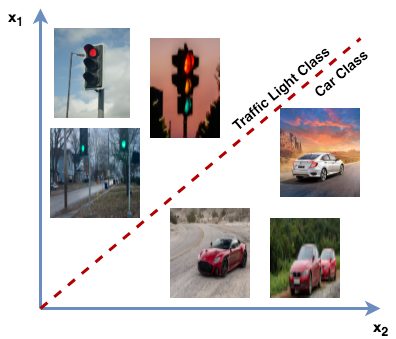
The discriminative model falls under the supervised learning branch. In a classification task, given that the data is labelled, it tries to distinguish among classes, for example, a car, traffic light and a truck.  Also known as classifiers, these models correspond image samples X to  class labels Y, and discover the probability of image sample belonging to class label .

They learn to model the decision boundaries among classes (such as cats, dogs and tigers ). The decision boundary could be linear or non-linear. The data points that are far away from the decision boundary (i.e. the outliers) are not very important. The discriminative model tries to learn a boundary that separates the positive from the negative class, and comes up with the decision boundary. Only those closest to this boundary are considered.

Discriminative models classify data points, without providing the model of how the points were generated.

In trying to classify a sample x belonging to class label y, the discriminative model indirectly learns certain features of the dataset that make its task easier.  For example, a car has four wheels of a circular shape and more length than width, while the traffic light is vertical with three circular rings. These features help the model distinguish between the two classes.

The discriminative models could be:

• Probabilistic
  • logistic regression
  • a deep neural network, which models P(Y|X)
• Non-probabilistic
  • Support Vector Machine (SVM), which tries to learn the mappings directly from the data points to the classes with a hyperplane.

Discriminative modelling learns to model the conditional probability of class label y given set of features x as P(Y|X).

Some of the discriminative models are:

• Support Vector Machine
• Logistic Regression
• k-Nearest Neighbour (kNN)
• Random Forest
• Deep Neural Network ( such as AlexNet, VGGNet, and ResNet )

Let’s study a few discriminative models and discover their prominent features.

Support Vector Machine

Support Vector Machine (SVM) is a non-parametric, supervised learning technique very popular with engineers for it produces excellent results with significantly less compute.  A Machine Learning algorithm, it can be applied to both classification (output is deterministic) and regression (output is continuous) problems. It is largely used in text classification, image classification, protein and gene classification.

The famous Deep Learning-based object-detection model, known as Regions with CNN (R-CNN), uses SVM to classify the objects in bounding boxes. In this paper, authors used class-specific Linear SVMs to classify each region in an image.

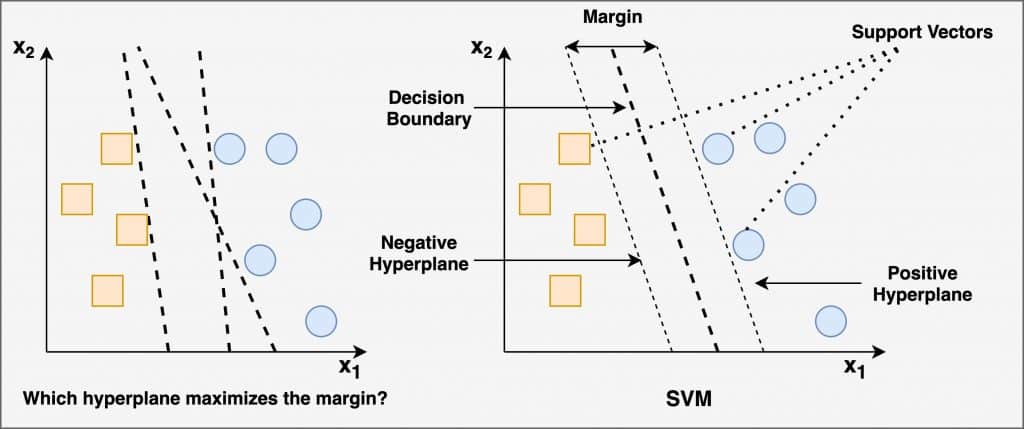
SVM can separate both linear and non-linear data points. A kernel-trick helps separate non-linear points. Having no kernel, the Linear SVM finds the hyperplane with the maximum margin-linear solution to the problem. The boundary points in the feature space are called support vectors (as shown in the  figure above). Based on their relative position, the maximum margin is derived and an optimal hyperplane drawn at the midpoint.

The hyperplane is N-1 dimensional, where N is the number of features  present in the given dataset. For example, A line will indicate the decision boundary if a dataset has two features (2d input space).

Why do we need a hyperplane with maximum margin?

The decision boundary with the maximum margin works best, increases the chance of generalization. Enough freedom to the boundary points reduces the chance of misclassification. On the other hand, a decision boundary with smaller margins usually leads to overfitting.

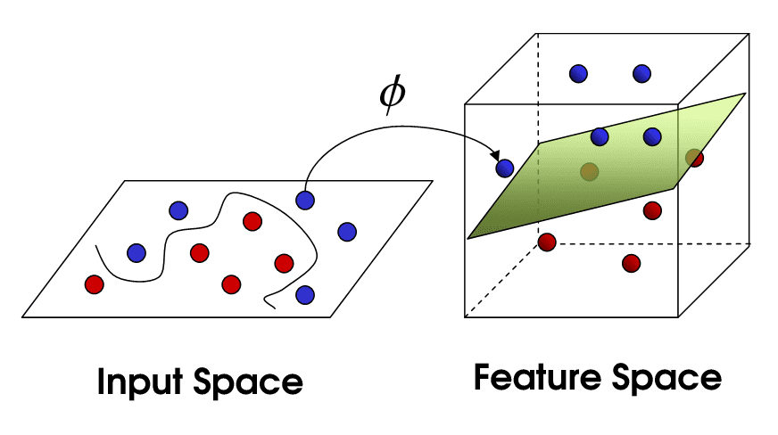
When the data points are not separated in a linear fashion, the Non-Linear SVM is used. A kernel function or a kernel trick helps obtain a new hyperplane for all the training data. As shown in the figure above, the input space is projected to a higher-dimensional feature space, such that the distribution of data points in the new hyperplane will be linear. Various kernel tricks, such as polynomial and radial basis function are used to solve nonlinear classification problems with SVM.

SVM can be used off-the-shelf. Just import the SVM module from the sklearn library.

from sklearn import svm

Random Forest

Like SVM, Random Forest also falls in the class of discriminative modelling. It is one of the most popular and powerful Machine Learning algorithms to perform classification and regression.  Random Forest became a hit in the Kaggle Community as it  helped win many competitions.

It is an ensemble of decision-tree models. Hence, to understand the Random Forest algorithm, you need to know  Decision Trees.

Microsoft trained a deep, randomized decision-forest classifier to predict 3D positions of body joints, from a single-depth image.  There was no temporal information, and hundreds of thousands of training images were used.

Now, what are Decision Trees?

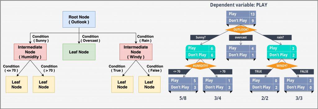
A Decision Tree is a non-parametric, supervised-learning algorithm, used in both classification and regression problems. However, it is predominantly used for classification. The decision tree progressively splits the data into smaller groups, based on certain  attributes, until they reach an end, where the data can be termed a label. Once it learns to model the data using labels, it tries to label the test set accordingly. It is a tree-structured classifier, consisting of a root node, an intermediate or decision node and a leaf node.

The data is represented in a tree structure, where each:

• internal node denotes a test on an attribute (basically a condition)
• branch represents an outcome of the test
• leaf node holds a class label

Decision Trees can broadly be categorised into two types:

• When the target variable is categorical (as shown in the figure above),
  • It predicts one of the two categories: play and do not play. 
  • Features include: outlook ( sunny, windy, rainy ), humidity, and windy. The Decision Tree learns from these features, and after passing each data point through each node, it ends up at a leaf node of one of the two categorical targets (play or do not play).
• When the target variables are continuous. For example, predicting the house price, based on different features of the house.

The splitting in decision trees could be:

• binary ( yes/no )
• multiway ( sunny, rainy, overcast )

(See the above figure)

The Decision Trees analyse all the data features to find the ones that split the training data into subsets to give the best classification results.  The training phase also determines which data attributes will be the root node, branches and intermediate. Data is split recursively till the tree reaches the leaf node. How the Decision Tree splits is governed by Gini Impurity or Entropy-the two criteria for selecting the intermediate ( conditions ) nodes.

The Decision Trees commonly use the Gini Impurity metric to create decision points that illustrate how finely the data has been split.

• When all the observations belong to the same label, it is a perfect classification, and the Gini Impurity is zero ( best ).
• When the observations are equally split between the labels, the Gini Impurity value is one ( worse ).

The decision tree module can be imported the sklearn library.

from sklearn.tree import DecisionTreeClassifier

Now apply all you learnt about the Decision Trees to know Random Forest.

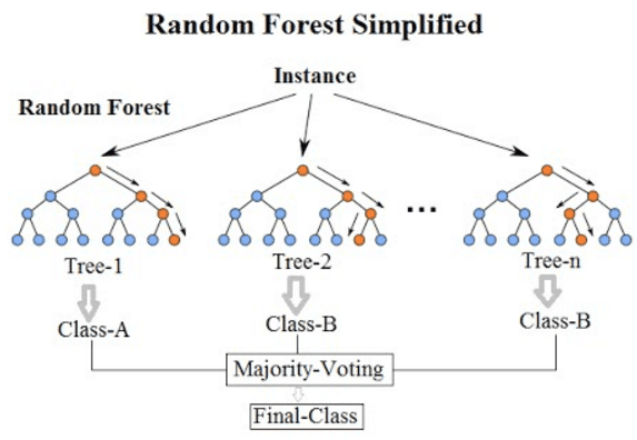
You can build the Random Forest classifier by combining multiple Decision Trees (as shown in the figure above). This brings the weak classifiers together and you end up with a more robust classifier. The derived model is not just stronger, but also more accurate and generalizes better ( improves variance ).

Import the Random Forest algorithm directly from the sklearn library.

from sklearn.ensemble import RandomForestClassifier

Because bootstrap samples train the Random Forest algorithm, random samples or data points can be drawn from the dataset, with replacement.

To ensemble the Decision Trees, Random Forest uses the bagging method. This one differs a bit though from conventional bagging. Instead of using all the features in a Random Forest, draw its random subsets to train each tree. The random feature selection allows the trees more independence. Each tree can then capture unique information from the dataset, which in turn improves the model’s accuracy and training time. After ensembling all the trees, it calculates the final output, using majority voting. The label with the maximum number of votes is termed the final prediction.

Deep Neural Network

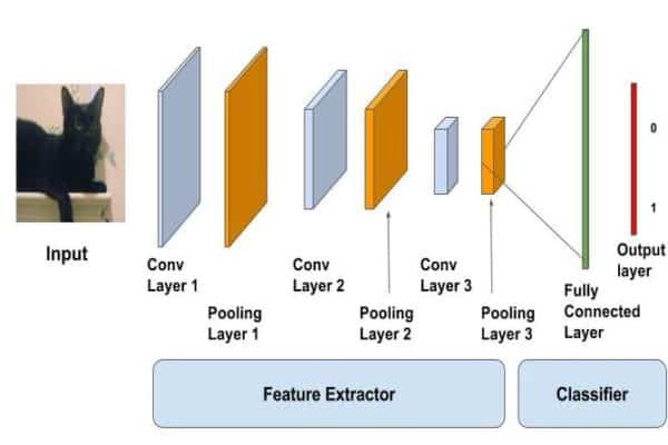
To understand deep neural networks, go back in time and first know Linear and Logistic Regression.

Linear Regression

Like  the name suggests, it is a regression model and a supervised learning algorithm. It thus inputs variables to output a continuous target like stock price, house-price predictions etc. Also, being a parametric Machine Learning algorithm, some of its parameters are learned during the training phase.

Linear Regression tries to find a linear decision boundary. The algorithm is quite simple and intuitive, and based on the equation of a line from two points: y = mx + b, where y is the dependent variable (predicted output y-axis), m is the slope of the line, x is the independent input variable (x-axis), and b is the y-intercept.

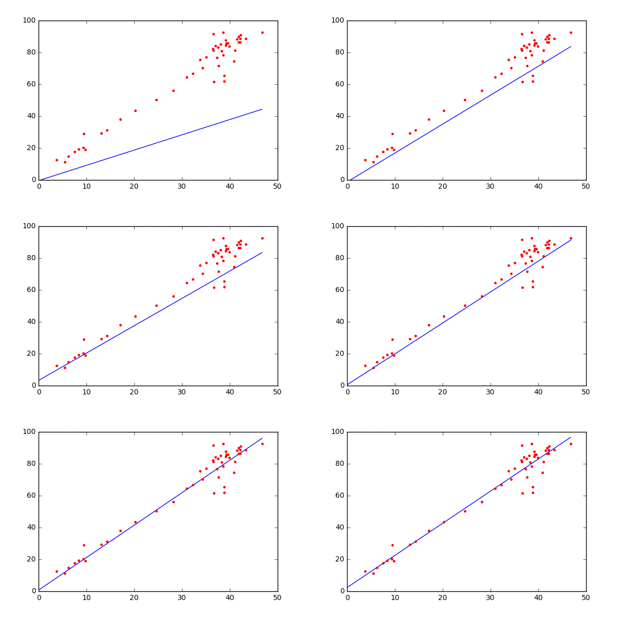
To simplify a bit, assume x is the area of a house (in square feet), while y is its price. The variables m and b are randomly initialized, and their values are updated till the loss (mean squared error) between the prediction () and the true value (y) is minimum (does not reduce further).

From Linear Regression to Logistic Regression

Logistic Regression

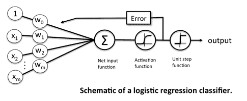
Logistic Regression is a parametric, supervised-learning algorithm used to solve classification problems. It is a generalized, linear Machine Learning-algorithm because the outcome always depends on the sum of the inputs and parameters. Don’t get confused by its name though. Addition of a  Logistic Function to Linear Regression built Logistic Regression. This was done to convert the target variable from continuous to deterministic, & bounded between 0 – 1.

The above figure shows the Logistic Function, also commonly known as the sigmoid activation function, which takes a real-valued number (x) and squashes it into a range between 0 and 1. It converts large negative numbers to 0 and large positive numbers to 1.

The modified linear regression equation can be given as , where is the sigmoid activation function. Like Linear Regression, here too, the parameters are updated by calculating the loss between the predicted output and true label. A binary cross-entropy function is used as the loss function.

Take the simple example of classifying cat and dog images. The Logistic Regression will take the input image x, and output a value between 0  and 1. Assume the true label for a cat is 0, and for a dog 1. When you input the cat image, the model predicts 0.2 as the output. The loss will then be computed between the true label: 0, and the predicted output: 0.2, and the parameters will be updated accordingly.

Import the Logistic Regression module from the sklearn library:

from sklearn.linear_model import LogisticRegression

Now dive straight into deep neural networks.

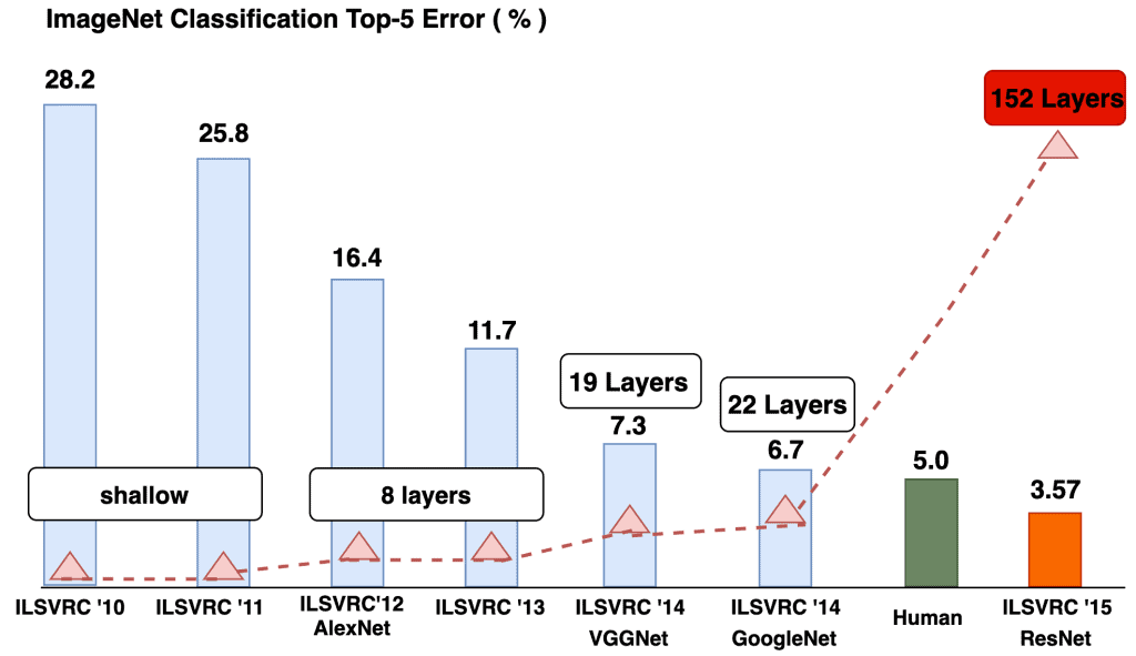
The above figure shows how much the Deep Neural Networks, popularly known as Deep Learning have progressed over the years. The classification regime has been benchmarked on the famous Imagenet Large Scale Visual Recognition Challenge ( ILSVRC ). You’ll find that the machine (ResNet) achieved a 3.57 top-5 classification error and surpassed the 5% error rate associated with human performance. Isn’t that amazing? The above figure made one more interesting point: As the number of layers in the neural networks increased, so did the model’s performance.

Deep Neural Networks ( DNNs ) are compelling, complex architectures that were designed to mimic the human brain. Since 2012, Convolutional Neural Networks ( CNNs ) outperformed hand-crafted descriptors and shallow networks by a large margin.

Hand-crafted descriptors ( LBP, SIFT ) are features, extracted using a manual, predefined algorithm to tune several parameters that are not well generalized over a dataset.

• Traditional hand-crafted descriptors explicitly extract features.
• In neural networks, features are inherently learned, as part of the training, which is more general across the data. No wonder, neural networks are known to be great feature extractors.

Shallow versus Deep Neural Networks: Shallow neural networks are not deep, having usually just that,one  hidden layer. A deep neural network may boast of having as many as 152 layers ( ResNet Architecture ).

Known to be excellent function approximators, neural networks have three types of layers: input, hidden, and output layer. The hidden layer is where all the magic happens.

• How does logistic regression relate to neural networks?  Basically, logistic regression is like a one-layer neural network. In contrast, deep neural networks are stacked logistic regressions.
• Remember, in logistic regression, you used the sigmoid activation function to learn non-linearity, which came with its own caveats. Deep neural networks however use more efficient pools of activation functions, such as ReLU, PReLU, and Swish. These outperformed the sigmoid and  further improved the performance of neural networks. Made them more than  just “deep.”

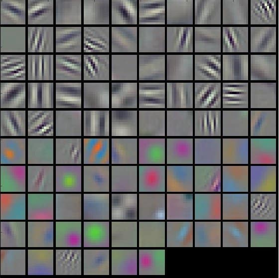
In DNN,  image classification tasks are performed first by the CNN layers, which learn the features. Next, the fully-connected layers aggregate those features and output a classification score ( probability of input image being a cat ). Of course, a lot more goes in before an image is successfully classified.

The initial layers in CNN (as shown  in the above visualization) learn low-level features like vertical, horizontal and diagonal s (local patterns). As you go deeper into the network, the features get more abstract (global patterns).

Comparison of Discriminative Models

Support Vector Machine ( SVM )

• SVM can be used for both classification and regression. It is a supervised learning algorithm.
• SVM performs better even if the training data is limited and the number of features more.
• It uses kernel tricks like Polynomial, RBF and Sigmoid to solve complex non-linear problems. You can not only define custom kernels, but also add some to achieve a more complex decision boundary.
• Use hinge loss for higher accuracy (it has its caveats though).
• SVM only supports binary classification. For multiclass classification, you  need to have multiple SVM models in place.
• Hyperparameters like soft-margin tuning helps  achieve sufficient accuracy.
• SVM is memory-efficient because here the maximum margin is derived from the support vectors, i.e., only a subset of data points.
• Being a non-probabilistic model, it does not output a probability for prediction or for probability estimates.
• You train on the CPU, which can be parallelized across cores. Large datasets obviously require more training time.
• A convex  objective function means there are no local optima, and the Lagrange multiplier comes into play instead of the gradient descent (used in DNNs).

Random Forest

• Random Forest can solve both classification and regression tasks. It is a supervised learning algorithm.
• Unlike SVMs, it can perform multiclass classification.
• Also, give a probability score for a prediction.
• They should be preferred when the dataset grows larger.
• Generalize well and do not overfit when multiple weak forests are combined.
• The training is slower if the number of forests is huge. However, if the training data size is large, we find it  trains faster than  SVM.
• It also supports implicit feature selection and tells you intuitively which features are important.

Deep Neural Network

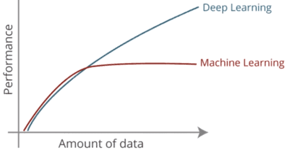
• Like the other two models, Deep Neural Networks ( DNNs ) also solve classification as well as regression problems.
• Use labels when applying DNNs  to supervised learning (eg, image classification). No labels needed but for unsupervised learning (eg, image generation).
• DNNs work well, especially when you have a lot of data.
• Unlike SVM, the objective function of DNN is non-convex, and more than one  local optima could exist. Gradient descent is used to optimize the training error.
• They are very compute-intensive: Higher the network depth, higher the compute requirement. You’ll need to train on  GPUs (graphical processing units).
• This method works best when trying to extract meaningful features from raw data. You need not depend on hand-crafted features like local binary patterns or a histogram of gradients.
• You need to really tune the hyperparameters of the neural network  in order to achieve the best results. They generalize well but when distributing the trained data.
• Used in millions of applications, the more  prominent ones being  computer vision, natural language processing/understanding, medical imaging, speech processing and time series.

So there isn’t one wonder algorithm that scores on all points. Which algorithm shall work depends on the dataset, type of problem, compute power, and the accuracy you expect to achieve.

Generative Modeling

Generative modelling defines how a dataset is generated. It tries to understand the distribution of data points, providing a model of how the data is actually generated in terms of a probabilistic model. (e.g., support vector machines or the perceptron algorithm gives a separating decision boundary, but no model of generating synthetic data points). The aim is to generate new samples from what has already been distributed in the training data.

Assume you have an autonomous driving dataset with an urban-scene setting. You now want to generate images from it that are semantically and spatially similar . This is a perfect example of a generative modelling problem. To do this, the generative model must understand the data’s underlying structure and learn the realistic, generalized representation of the dataset, such as the sky is blue, buildings are usually tall, and pedestrians use sidewalks.

The above image is an example of sample generation, using generative modelling. The goal is to input training samples with probability distribution P_data, and learn a distribution such that: When you sample from the distribution P_model,,  it generates realistic observations that represent the true distribution.

To generate such training samples, you need a training dataset, which consists of unlabelled data points. Each data point has its own features, such as individual pixel values (image-domain ) and a set of vocabulary (text-domain). This whole process of generation is stochastic and influences the individual samples generated by the model.

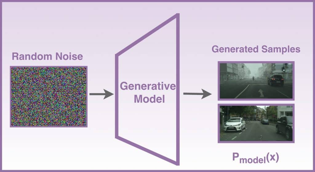
Generative models, you know by now, try to learn the probabilistic distribution of the training data. This helps them represent the data more realistically. In the above figure, the generative model learns to generate urban-scene images, taking a random noise as a matrix or vector. Its task is to generate realistic samples X, with probability distribution similar to P_data (original data from the training set). The noise adds randomness to the model and ensures that the images generated are diverse.

Generative modelling learns to approximate p(x), which is the probability of observing observation x.

Types of Generative Models

Here are some of the popular ones:

• Naive Bayes
• Hidden Markov Models
• Autoencoder
• Boltzmann Machines
• Variational Autoencoder
• Generative Adversarial Networks

Let us now understand two of these models: Autoencoder and Variational Autoencoder. This section tells you about unsupervised learning (without labels).

Autoencoder

This neural network is primarily used to learn data compression in an unsupervised way. The goal of an Autoencoder is to learn a generalized latent representation (encoding) of a dataset, just like the PCA. It has also been widely adopted to solve self-supervised learning problems. The Autoencoder network is segmented into two blocks:

• The encoder compresses the high-dimensional input data into a low-dimensional regime, also known as latent space representation, preserving all relevant information.
• The decoder functions opposite to an encoder, decompressing the low-dimensional representation back to its original high-dimensional input.

In a traditional Autoencoder, as shown in the figure above:

• Use an activation function to try and recreate the original image, after some generalized non-linear compression.
• Minimize the loss between the input image and the reconstructed (predicted) output, using euclidean distance as the loss function.
• Perform this process iteratively, until you reach a point where the loss is minimal, and the reconstructed output is the same as  the input.

This trains the network to find the best weights for the encoder as well as the decoder.

Applications of autoencoder include:

• denoising images
• dimensionality reduction
• clustering
• recommender systems
• image inpainting

They can also generate data; the vanilla Autoencoder can’t though, due to some caveats discussed in the next section.

A deep encoder-decoder architecture called SegNet was developed, especially for multi-class, pixel-wise segmentation on the urban-road scene dataset. The Computer Vision Group at the University of Cambridge then published their work. Try out their demo!

It is important to note that an Autoencoder is not purely a generative model. Its latent space is not modelled to generate new data points, given a random normal vector. Hence, to make them generative,  move to Variational Autoencoders. Many variants exist, like denoising, stacked etc. Instead of dwelling on details of these variants, let’s try  to understand what exactly is a Variational Autoencoder.

Variational Autoencoder

Variational Autoencoder (VAE) is a generative model that enforces a prior on the latent vectors so that they all lie on the gaussian plane or have a Gaussian profile (prior on the distribution of representations). Instead of mapping the image on a point in space, the VAE encoder maps the image onto the whole distribution (multivariate normal or gaussian distribution). It then randomly samples a point from that distribution to reconstruct the image. This helps it learn how the data is distributed.

In the above figure, digit 6 is encoded in two ways:

• On the left, the digit 6 is mapped to a single point (traditional autoencoder). Consider an image represented by a column of numbers,where the column’s size equals the latent space dimension.
• On the right, the digit 6 is mapped to a Gaussian distribution, as you explicitly learned the distribution.

You might  question why traditional Autoencoders did not generate new samples?

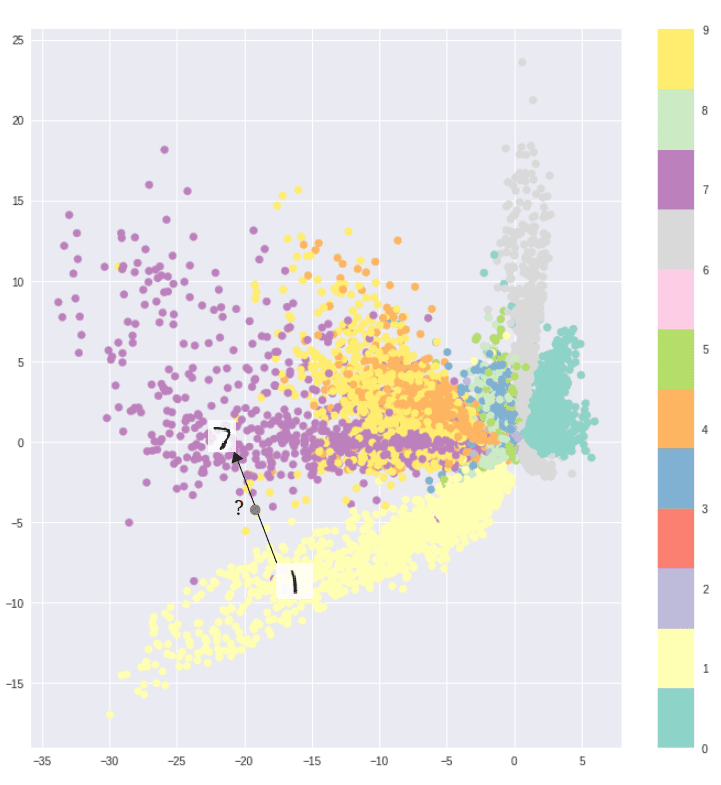
That’s because:

1. The latent space in Autoencoders was irregular and not continuous. It was almost impossible to know which random point to pick and decode from the latent space to generate a realistic image, as there were many gaps in the clusters. If you picked a point from the gap and passed it to the decoder, it might give an arbitrary output that does not resemble any class.
2. Also, the distribution of points from the latent space is not defined properly, for it mapped each image directly to one point. Whereas, each image in a VAE is mapped to a multivariate gaussian or normal distribution, whose inherent property is to make the latent vectors continuous.

Input an image in the VAE encoder. It encodes it into two separate vectors: mean and logarithm of the variance, corresponding to the latent space variables. If you take a  random sample from the distribution and pass it to the decoder next, it reconstructs the image. 

By training such a model:

• You ensure the latent space representation is continuous
• Learn a pool (100 pools in case of a VAE that trained on 100 classes), such that they are in a well-defined region.

Unlike an Autoencoder, VAE not only ensures that the two close points in latent space give identical outputs, but also that a point sampled from here results in a meaningful output.

What makes the Variational Autoencoder a generative model? Once the model is trained, at the time of testing, you basically get rid of the encoder and sample a point from the normal distribution. This when passed  through the decoder generates diverse, realistic images.

You may still wonder, what are we optimizing in a VAE? Well, unlike traditional Autoencoders, VAE optimizes a reconstruction loss (euclidean) plus a latent loss (KL-divergence). The KL-divergence measures the divergence between a pair of probability distributions. The latent loss forces the latent representation to be continuous, and confines the pools learned by the network in one  region.This ensures the distribution learned by your model is well-defined and similar to normal distribution.

Variational Autoencoder (VAE) has also been used in a Reinforcement Learning (RL) paper called Improving Zero-Shot Transfer in Reinforcement Learning. The authors run the RL agent on the VAE’s compressed representation, instead of the entire input space. The RL rewards are sparse and take a long time to train, so VAE.

Generative Adversarial Network

• Though the VAE model takes from both the generative and inference models, and learns the underlying data distribution in an unsupervised way, the images generated by it are blurryGenerative Adversarial Network ( GAN ) yields sharp and perceptually better images.
• In VAE,  the lower variational bound is optimized. No such assumption exists in GAN. In fact, GANs do not deal with any explicit probability-density estimation.

The failure of VAE in generating sharp images implies that the model is unable to learn the true posterior distribution,

 i.e., P(x|z), where x is the generated sample, and z is the latent-space representation expected to be close to a normal distribution.

Our next post dwells on Generative Adversarial Network quite comprehensively and gives you an intuitive understanding of GAN architecture, adversarial loss function, and its training strategy. You also code a vanilla GAN to generate fashion images in PyTorch and TensorFlow. Do give it a read!

Generative vs Discriminative Modeling

• Both Generative (G) and Discriminative (D) can be used for classification.
• G models work with both  supervised and unsupervised learning. But D models are only used for supervised learning problems.
• The goal of the D model is to estimate the conditional probability P(Y|X). In contrast, the G model learns to approximate P(X)  and P(X|Y) in an unsupervised setting, then deduces P(Y|X) in a supervised setting.
• D models learn a linear and non-linear decision boundary, using the data points and their respective labels, without  knowing how the data was generated. In learning to model the probability distribution of the data, G models get to  understand the data’s underlying characteristics.
• In a supervised setting, D models are known to outperform G models. Especially, when G models do not fit the data well.
• G models can provide rich insights about  the data, when you do not  have labels.

Conclusion

Congratulations on making this far. That’s commendable! Here’s a quick summary.

You now have a comprehensive understanding of the theory as well as the  working of both Discriminative and Generative modelling, which are the two eminent models in  Machine Learning. Even prominent latent-variable models for each were discussed. A comparative analysis of the two models must have helped you gain a better understanding of their strengths and weaknesses.

Along the way, we provided details of resources and links for a comprehensive learning experience.

Key takeaways of Generative and Discriminative models:

1. Both can be used for classification.
2. Discriminative models are only for supervised learning problems, whereas Generative models  apply to both supervised and unsupervised learning.
3. Discriminative models are known to outperform Generative models. Especially, when Generative models do not fit the data well.
4. Generative models can provide rich data insights , when you do not have any labels.

Hope this post helps you get closer to your goal post! Do share your experience and feedback via the comments section.