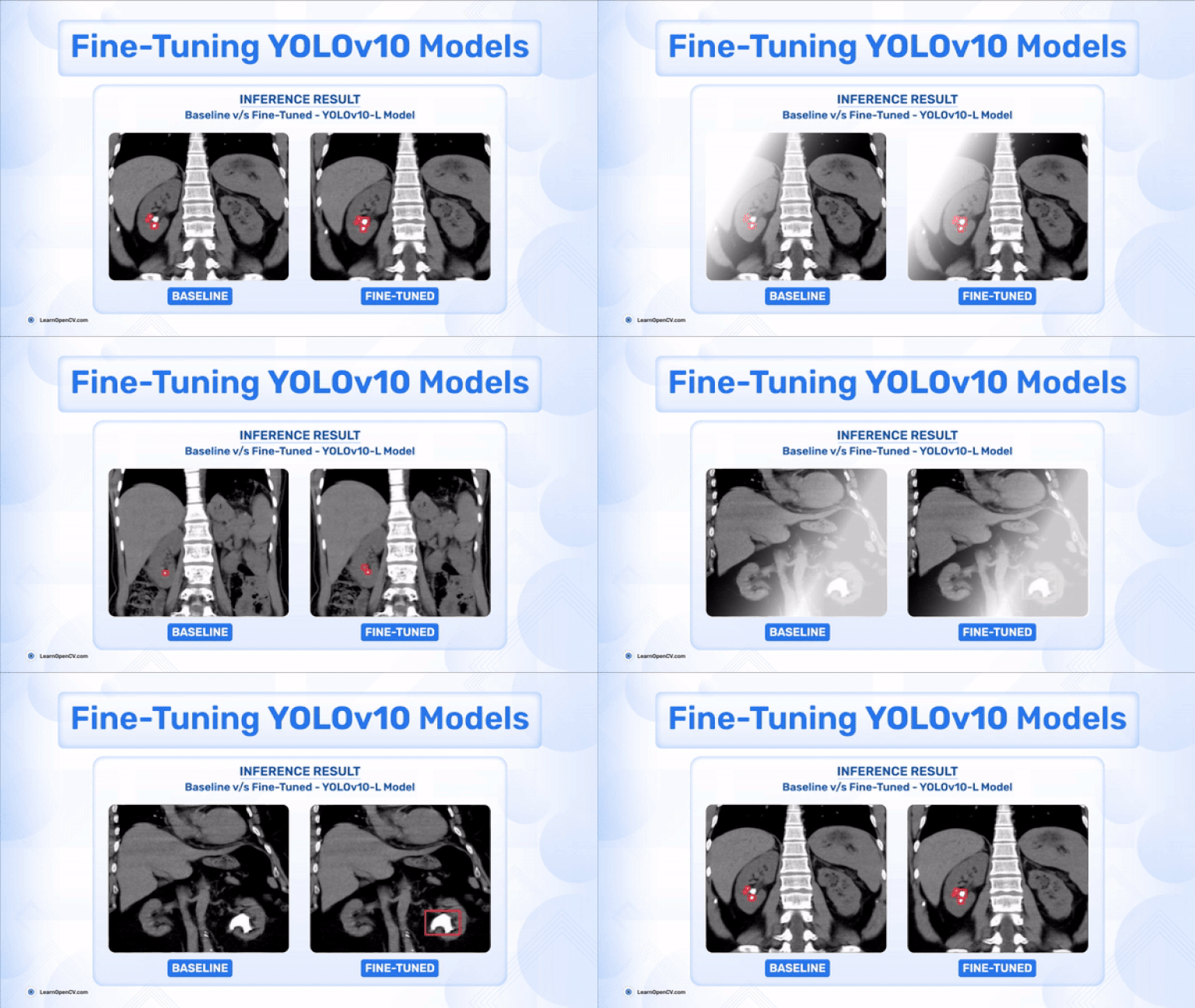
Fine-Tuning YOLOv10 Models on Custom Dataset

Fine-tuning YOLOv10 models for enhancing kidney stone detection, significantly reduces diagnosis time from 15-25 minutes per report to processing ~150 reports per second. Targeting medical researchers, healthcare professionals, and AI companies, this research work was able to yield a mAP50 of 94.1 through data-centric techniques without altering the model architecture.

fine tuning yolov10 models custom dataset kidney stone detection medical diagnosis treatment medical image analysis

The findings focus on improving data quality to tackle false positives and misclassifications. SCROLL BELOW to the concluding part of the article or click here to see the experimental results right away.

NMS Free Training: Is it really effective?
Kidney Stone Detection: Dataset Visualization
Code Walkthrough
Baseline Training Performance Metrics – YOLOv10 Models
Baseline Inference Visualization: YOLOv10L Model
Fine-Tuning YOLOv10 Models: A Data Centric Approach
Performance Metrics: After Fine-Tuning YOLOv10 Models
Experimental Inference Results: Baseline v/s Fine-Tuned
Key Takeaways
Conclusion
References

NMS Free Training: Is it really effective?

Ao Wang, Hui Chen et al [1] recently released their implementation of YOLOv10. In their paper, the authors integrated the concept of NMS Free Training into the YOLO detection pipeline. However, the question is – what is it and how does it even make a difference?

To understand this, it is important to look at what Non-Maximum Suppression (or) NMS is, and how it works. In the paper by Juan Terven and Diana Cordova-Esparza [2], the working algorithm for NMS has been shown.

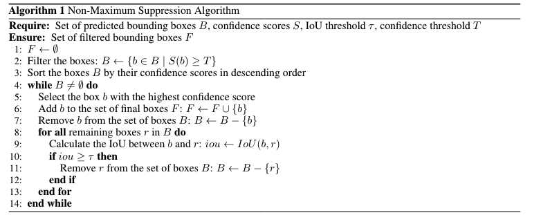
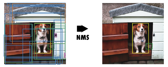
nms non maximum suppression algorithm — **FIGURE 1:** Non-Maximum Suppression Algorithm [2]

They explain it as a post-processing technique used in object detection algorithms to reduce the number of overlapping bounding boxes and improve the overall detection quality. NMS can filter out redundant and irrelevant bounding boxes, keeping only the most accurate ones. FIGURE 2 below shows a better visualization of this algorithm.

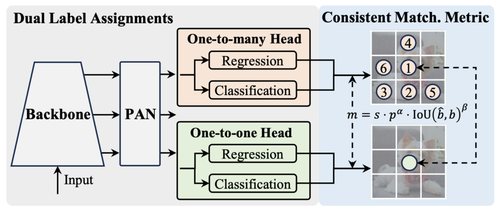
nms non maximum supression algorithm visualization — **FIGURE 2:** Visual Representation of Non-Maximum Suppression – from Paper [2]

However, the authors of YOLOv10 have used an NMS-free approach for object detection in their paper. They felt that the previous variants of YOLO models heavily relied on NMS for post-processing, which caused suboptimal inference efficiency during deployment. Dual Label Assignments and Consistent Matching Metrics were preferred for this. To understand this better, let’s examine the architecture in FIGURE 3.

dual label assignment fine tuning yolov10 — **FIGURE 3:** Consistent Dual Assignments for NMS-free Training – from Paper [1]

Dual Label Assignments

Traditionally, one-to-many assignments provide rich supervision but require non-maximum suppression (NMS) post-processing. In contrast, one-to-one assignments are simpler and NMS-free but offer weaker supervision, impacting accuracy and convergence. To address these issues, dual label assignments introduce a secondary one-to-one head alongside the traditional one-to-many head. Both heads operate jointly during training, enhancing the model with comprehensive supervision from the one-to-many setup. Only the more efficient one-to-one head is used for inference, reducing computational overhead. This method leverages top-one selection in one-to-one matching, performing comparably to Hungarian matching but with reduced training complexity.

Consistent Matching Metrics

The consistent matching metric is designed to standardize the evaluation of both one-to-one and one-to-many approaches, ensuring harmony between them. It uses a formula $m(\alpha, \beta) = s \cdot p^\alpha \cdot \text{IoU}(\hat{b}, b)^\beta$ , where $p$ is the classification score, $\hat{b}$ and $b$ are the predicted and actual bounding boxes, respectively, and $s$ indicates the spatial alignment of the prediction’s anchor point. The parameters $\alpha$ and $\beta$ balance the influence of classification accuracy and bounding box precision. The consistent matching metric helps align the supervisory signals of both heads by employing uniform hyperparameters, leading to better sample quality during inference and minimal supervision gaps. The effectiveness of this alignment is confirmed by improved consistency in one-to-one matches within the top results of one-to-many outputs after training.

Kidney Stone Detection: Dataset Visualization

In this research article, the Kidney Stone Detection dataset from Kaggle has been used to fine-tune YOLOv10 models. Let’s also examine a few samples from this dataset.

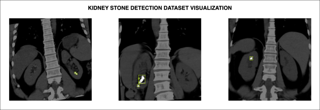
kidney stone detection system fine tuning yolov10 medical diagnosis — **FIGURE 4:** Kidney Stone Detection Dataset Visualization

As shown in FIGURE 4, this is a single class dataset, and has bounding box annotations for kidney stones of varying sizes and shapes. The specifications are given below:

Train: 1054 images
Test: 123 images
Valid: 123 images

Hence, this dataset contains 1300 images in total.

Code Walkthrough

In this section, we can understand the setup process for YOLOv10 models. You can also download the notebook used in this research.

Download Code To easily follow along this tutorial, please download code by clicking on the button below. It's FREE!

Click here to download the source code to this post

Initially, the YOLOv10 repository needs to be cloned into your local development environment. Before that, make sure to get back to your root directory, and then use the code below to clone the repository.

HOME = os.getcwd()
print(HOME)

!pip install -q git+https://github.com/THU-MIG/yolov10.git

NOTE: At the time of publishing this research work, there are 6 variants of YOLOv10 models. Based on your requirements, download the model of your choice.

!mkdir -p {HOME}/weights
!wget -P {HOME}/weights -q https://github.com/THU-MIG/yolov10/releases/download/v1.1/yolov10n.pt
!wget -P {HOME}/weights -q https://github.com/THU-MIG/yolov10/releases/download/v1.1/yolov10s.pt
!wget -P {HOME}/weights -q https://github.com/THU-MIG/yolov10/releases/download/v1.1/yolov10m.pt
!wget -P {HOME}/weights -q https://github.com/THU-MIG/yolov10/releases/download/v1.1/yolov10b.pt
!wget -P {HOME}/weights -q https://github.com/THU-MIG/yolov10/releases/download/v1.1/yolov10x.pt
!wget -P {HOME}/weights -q https://github.com/THU-MIG/yolov10/releases/download/v1.1/yolov10l.pt
!ls -lh {HOME}/weights

From here, you just need to alter the PATH variables in your data.yaml file and run the following command-line argument to start the training process.

!yolo task=detect mode=train epochs=100 batch=16 plots=True \
model=/weights/yolov10l.pt \
data=/data.yaml

That’s it. This is all you need to get this model up and ready for training.

Baseline Training Performance Metrics – YOLOv10 Models

Alright, so how do these models perform without any type of fine-tuning? Let’s have a look at the baseline results. In this initial experiment, all the variants of YOLOv10 models were used to train on the Kidney Stone Detection dataset directly. The graph below shows the variation in mAP50 values achieved by all these models.

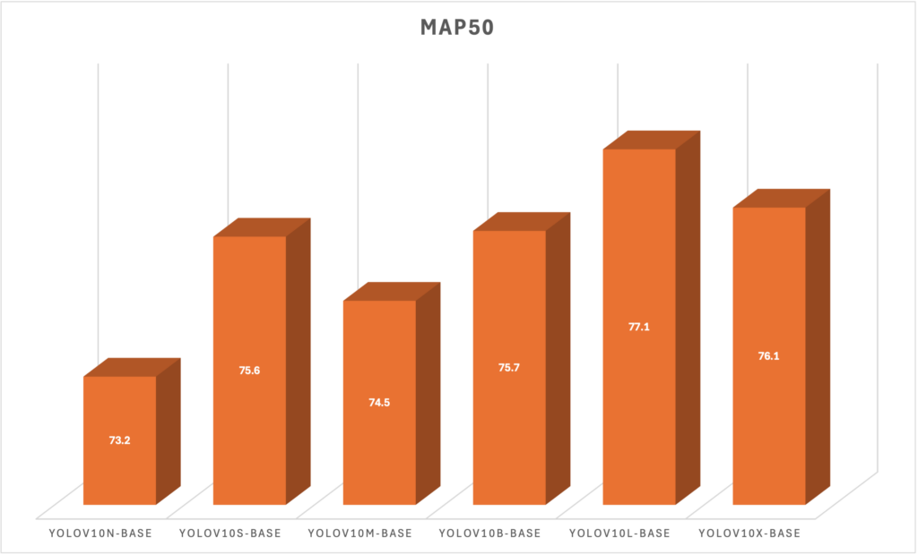
yolov10 models baseline results kidney stone detection system — **FIGURE 5:** Baseline Performance Metrics for YOLOv10 Models

From the above FIGURE 5, it is clear that as a baseline benchmark, all the variants achieved more than 70 mAP50. From the trend shown in the same FIGURE, it can also be inferred that the YOLOv10-L model achieved the highest mAP50 value of 77.1. Given below is the detailed analysis obtained from the training run for the large model.

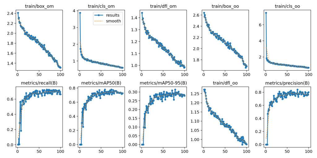
yolov10 baseline results map kidney stone detection — **FIGURE 6:** Baseline Performance – YOLOv10-L – 100 EPOCHS

Baseline Inference Visualization: YOLOv10L Model

From the previous section, we inferred that the YOLOv10-L model achieved an mAP50 value of 77.1. The first question that comes to mind is why this model didn’t get a much higher score.

In this section, let’s have a comprehensive look at the inference results obtained from this model and compare the ground truth annotations with the predictions. This analysis will allow us to understand where the model fails exactly.

Sample 1: Large Kidney Stones

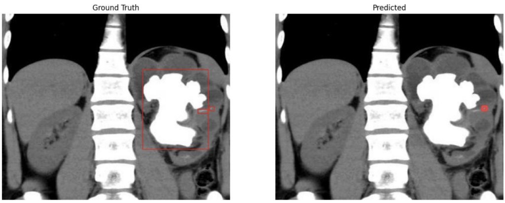
yolov10 missed detection kidney stone detection computer vision — **FIGURE 7:** Missed Detection – Large Kidney Stone

OBSERVATIONS: In this sample, the model could not detect the large kidney stone from the input image. The shape of the stone is comparatively larger than the usual ones, and the shape of the stone also looks irregular.

Sample 2: Small Kidney Stones

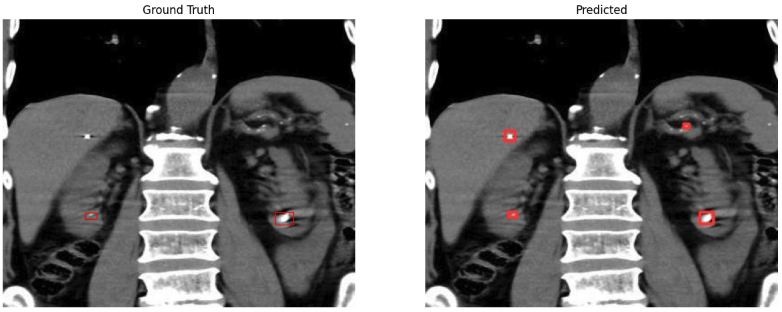
yolov10 missed detection small kidney stone detection computer vision fine-tuning yolov10 — **FIGURE 8:** Missed Detection – Small Kidney Stone

OBSERVATIONS: On the flip side, a few samples contain white-pixel artifacts that resemble the appearance of smaller kidney stones. In this sample, it can be observed that the model confused a white-pixel artifact for an actual stone. This is not acceptable, specifically in medical diagnosis.

Sample 3: Kidney Stones of Varying Sizes in the Same Image

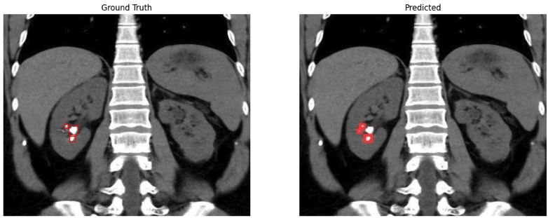
yolov10 detecting stones of varying sizes kidney stone detection medical diagnosis computer vision fine-tuning yolov10 — **FIGURE 9:** Missed Detection – Kidney Stones of Varying Sizes

OBSERVATIONS: In samples such as the one shown above, we can observe that there are kidney stones of varying sizes and shapes within the same sample. This poses a threat to any detection model. Here, the model failed to detect the comparatively bigger stone. Not only that, but the model also confused a white-pixel artifact for an actual small stone. This, again, is not acceptable.

Fine-Tuning YOLOv10 Models: A Data Centric Approach

In the previous section, we examined three samples in which the model failed to detect kidney stones accurately. Let’s now explore a few data-centric approaches that can mitigate these issues and allow the YOLOv10-L model to achieve a much higher mAP50 value.

ROI Sampling

From the observations in a few of the initial inference samples, it can be seen that the model could not detect a few larger irregular stones from the validation set. There are also other structures within the kidney image that resemble a large stone. In such cases, it is important to implement this technique known as ROI Sampling.

The basic idea here is to sample the Region of Interest (or) ROI, in this case, the large stone, and introduce unannotated instances of it within the same sample. For a start, the ROI sample can be placed:

outside the kidney structure
partially on the kidney and background
where a part of it is seen, and the other half is hidden

This allows the model to gain a contextual understanding of the shape and location of such stones, and prevents it from misclassifying (or) missing large stones within the kidney.

VISUALIZATION

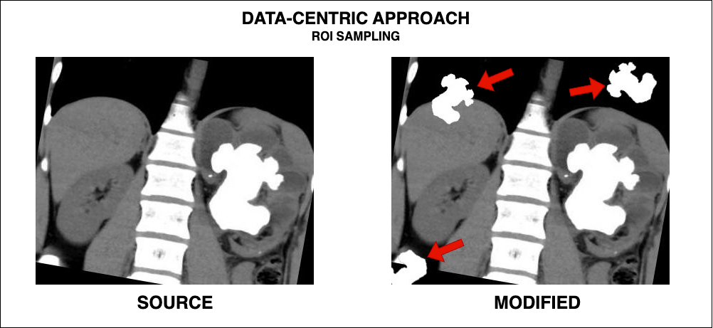
fine tuning yolov10 data centric approach roi sampling fine tuning technique kidney stone detection computer vision fine-tuning yolov10 — **FIGURE 10:** Data-Centric Approach – ROI Sampling

NOTE: All the image manipulations done as part of this work were manually done on Adobe Photoshop for Mac using the Quick Selection Tool.

Random Salt / Pepper Noise

The second problem that the model struggled with was detecting really small stones. Here, the white-pixel artifacts within the samples are to be blamed. Hence, if we introduce more unannotated white artifacts within such samples, the model will learn to predict against it.

For this, white artifacts of size 4px with 50% opacity were randomly introduced in a few samples that contained really small stones. It was also ensured that it followed a wide spread with the sample.

VISUALIZATION

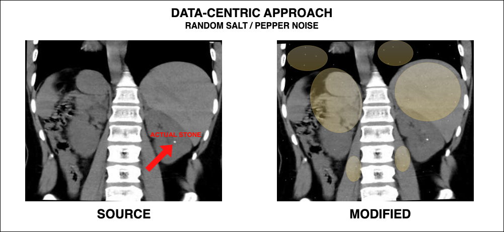
yolov10 data centric fine tuning technique random salt pepper noise small kidney stone detection medical diagnosis computer vision fine-tuning yolov10 — **FIGURE 11:** Data-Centric Approach – Random Salt / Pepper Noise

In FIGURE 11, the sample on the left represents the image where the actual stone has been highlighted. On the right, the highlighted regions show the parts where the Salt / Pepper Noise has been introduced. It can also be seen that the white artifacts are of the same size as the actual stone, with the opacity decreased by half. By doing this, we can teach the model to gain confidence in detecting actual small stones.

Contextual ROI Sampling + Contextual Salt / Pepper Noise

The last problem concerns stones of varying sizes and shapes within the same sample. Now, this is a tricky one. In this case, there might be a need to add two types of image manipulations in the same sample.

Here, both 4px white-artifacts with varying opacity levels from 50% – 75% were added in three parts of the sample, similar to the locations mentioned in the ROI Sampling section. The same was done for the ROIs as well.

VISUALIZATION

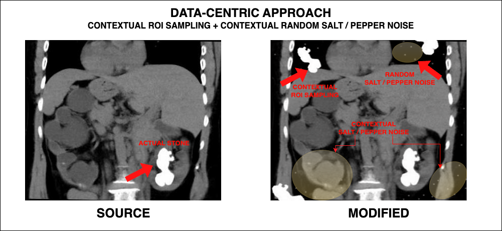
fine tuning yolov10 data centric approach contextual roi sampling contextual random salt pepper noise small and large kidney stone detection — **FIGURE 12:** Data-Centric Approach – Contextual ROI Sampling + Random Salt / Pepper Noise

From the above FIGURE 12, it can be seen that we are giving the model with more contextual information on the location of stones, and their variations.

NOTE: In this experiment, these techniques were applied on about 10 samples taken from the training set of the dataset, and then added back into the same training set after modification. None of the annotation files were touched.

Performance Metrics: After Fine-Tuning YOLOv10 Models

In the previous section, a few data-centric techniques were discussed. But the question now is: Does it make any difference? The series of experiments shown below will answer this.
NOTE: All the runs shown in this research article were done on an Nvidia RTX A5000 GPU with 24GB vRAM.

Experiment 1: Modified Dataset + 100 EPOCHS

In this initial experiment, the modified dataset containing the newly modified samples was used to train the YOLOv10L model for 100 EPOCHS. Here are the results from this experiment.

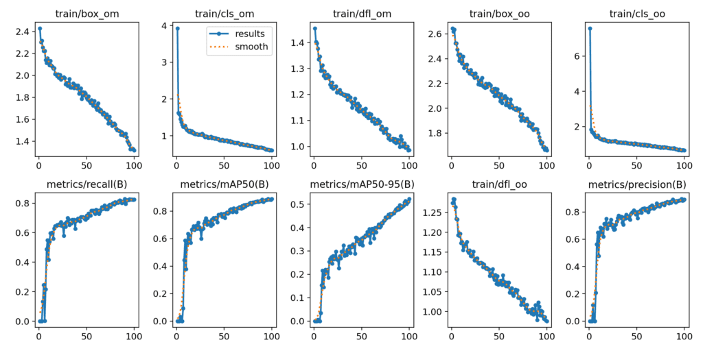
fine tuning yolov10 kidney stone detection 100 epochs modified dataset medical diagnosis computer vision — **FIGURE 13:** Performance after Fine-Tuning: Modified Dataset + 100 EPOCHS

The results shown in FIGURE 13 instantly show a massive performance boost in mAP50 value from 77.1 (initial baseline) to 89.0! It also looks like the model can do much better; let’s try training it for longer.

Experiment 2: Modified Dataset + 150 EPOCHS

In this experiment, the number of training EPOCHS has been increased from 100 to 150. FIGURE 14 shows the newly obtained results.

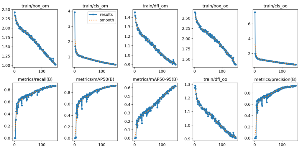
fine tuning yolov10 kidney stone detection 150 epochs modified dataset medical diagnosis computer vision — **FIGURE 14:** Performance after Fine-Tuning: Modified Dataset + 150 EPOCHS

An increase in the mAP50 value from 89.0 (from Experiment 1) to 92.3 has been observed. Let’s push this even harder, shall we?

Experiment 3: Modified Dataset + 200 EPOCHS

In this final experiment, the number of training EPOCHS has been increased to 200. Let’s have a look at the results from this run.

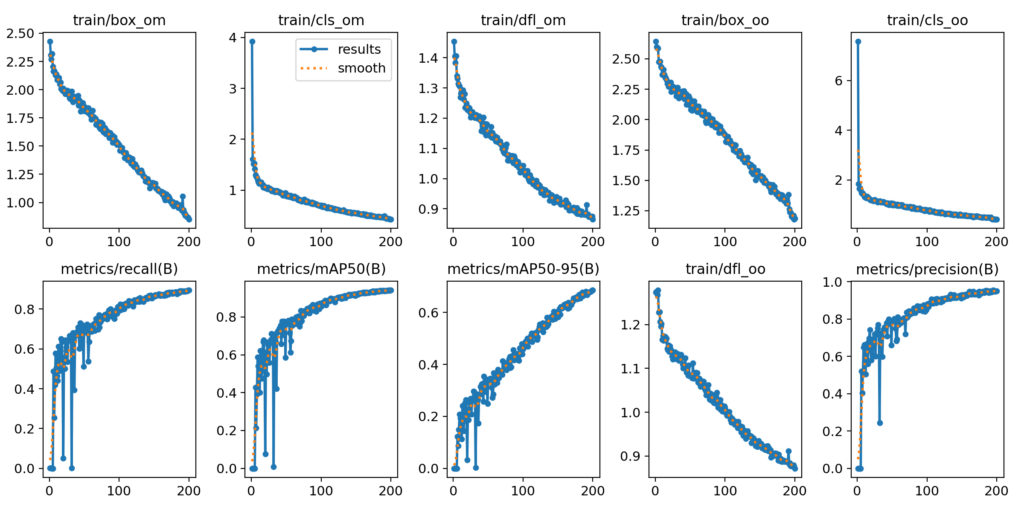
fine tuning yolov10 kidney stone detection 200 epochs modified dataset medical diagnosis computer vision — **FIGURE 15:** Performance after Fine-Tuning: Modified Dataset + 200 EPOCHS

FIGURE 15 shows that this run yielded an mAP50 value of 94.1. How crazy is that?

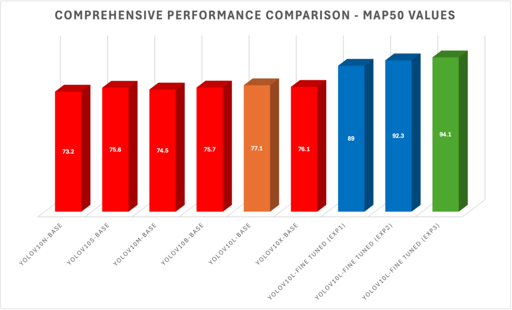
fine tuning yolov10 models comprehensive performance comparison map50 values with baseline and fine model yolov10l medical diagnosis computer vision kidney stone detection — **FIGURE 16:** Fine-Tuned Performance Metrics for YOLOv10 Models

In FIGURE 16 above, a comprehensive comparison of the mAP50 values of the baseline results with the fine-tuned YOLOv10 results has been shown.

Hence, with this series of experiments, the highest mAP50 value achieved is 94.1!

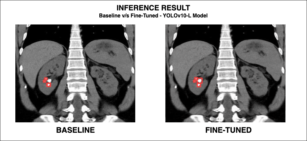
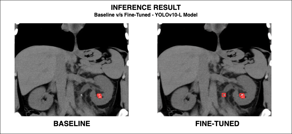
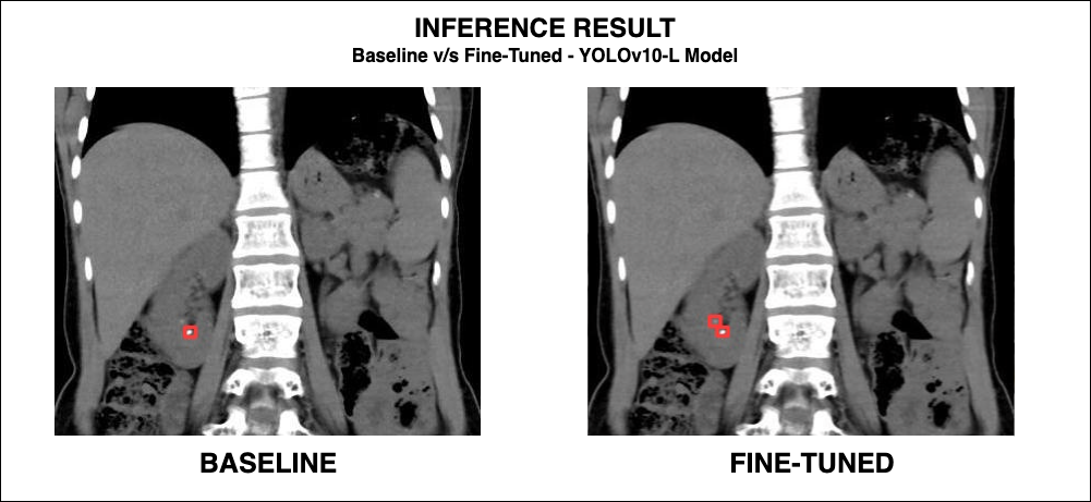
Experimental Inference Results: Baseline v/s Fine-Tuned

In the previous section, a comprehensive comparison in terms of mAP50 values was shown and discussed. But, how do these models perform in the real-world?

Inference Result 1

fine tuning yolov10 baseline vs fine tuned comparison small kidney stone detection computer vision medical diagnosis yolov10l fine-tuning yolov10 — **FIGURE 17:** Inference Result – Baseline v/s Fine-Tuned – 1

Inference Result 2

fine tuning yolov10 baseline vs fine tuned comparison small kidney stone detection computer vision medical diagnosis yolov10l — **FIGURE 18:** Inference Result – Baseline v/s Fine-Tuned – 2

Inference Result 3

Inference Result 4

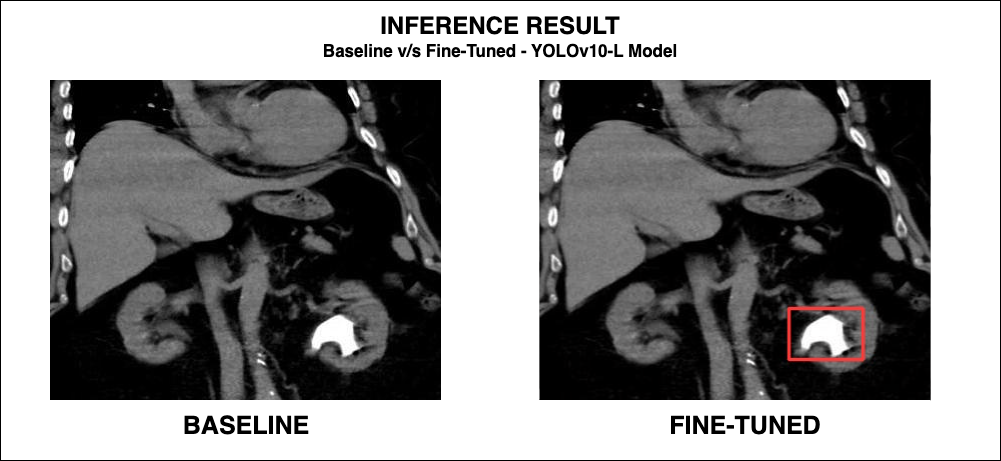
fine tuning yolov10 baseline vs fine tuned comparison large kidney stone detection computer vision medical diagnosis yolov10l fine-tuning yolov10 — **FIGURE 20:** Inference Result – Baseline v/s Fine-Tuned – 4

In this section, FIGURE 17, FIGURE 18, FIGURE 19, FIGURE 20 show that the fine-tuned model is able to detect stones of varying shapes and sizes. Interesting results, right? SCROLL UP or have a look at the code walkthrough section to explore the intricate fine-tuning procedure.

Key Takeaways

The following points summarize the key research findings on improving YOLOv10 models for better object detection performance and efficiency.

Fine-tuning YOLOv10 models on the Kidney Stone Detection dataset significantly improved detection efficiency, achieving an impressive mAP50 value of 94.1, highlighting the potential of YOLOv10 in medical diagnosis.
Implementing data-centric approaches such as ROI Sampling, Random Salt / Pepper Noise, and Contextual ROI Sampling with noise introduction improved model performance, addressing issues like misclassification and missed detections of kidney stones.
The adoption of Dual Label Assignments and Consistent Matching Metrics in YOLOv10’s NMS-free approach led to enhanced inference efficiency and reduced computational overhead, contributing to more accurate and faster object detection.

Conclusion

This research article explores a data-centric approach to fine-tuning YOLOv10 models. Through a series of experiments, including increased training epochs, the fine-tuned YOLOv10 models showed a substantial performance increase, with the mAP50 value rising from 77.1 in baseline tests to 94.1 after fine-tuning, demonstrating the effectiveness of the applied techniques.

References

[1] Wang, A., Chen, H., Liu, L., Chen, K., Lin, Z., Han, J., & Ding, G. (2024). Yolov10: Real-time end-to-end object detection. arXiv preprint arXiv:2405.14458.

[2] Terven, Juan, and Diana Cordova-Esparza. “A comprehensive review of YOLO: From YOLOv1 to YOLOv8 and beyond.” arXiv preprint arXiv:2304.00501 (2023).

[3] YOLOv10 Official Repository – GitHub

Download Code To easily follow along this tutorial, please download code by clicking on the button below. It's FREE!

Click here to download the source code to this post