Fine Tuning TrOCR – Training TrOCR to Recognize Curved Text

TrOCR (Transformer based Optical Character Recognition) models are some of the best performing OCR models. In our previous article, we analyzed how well they perform on single line printed and handwritten text. However, like any other deep learning model, they have their limitations. TrOCR does not perform well on curved text out of the box.  This article will take the TrOCR series a step further by fine tuning TrOCR model on a curved text dataset.

We know from the previous article that TrOCR cannot recognize text on curved and vertical images. Those images were part of the SCUT-CTW1500 dataset. We will train the TrOCR model on this dataset and run inference again to analyze the results. This will provide us with a comprehensive idea of how far we can push the boundaries of the TrOCR models for different use cases.

We will use the Hugging Face Trainer API for training the model. To complete the entire process, the following steps must be followed:

• Prepare and analyze the curved text images dataset.
• Load the TrOCR Small Printed model from Hugging Face.
• Initialize the Hugging Face Sequence to Sequence Trainer API.
• Define the evaluation metric
• Train the model and run inference.

The Curved Text Dataset

The SCUT-CTW1500 dataset (referred to as CTW1500 from here on) contains several thousand images of curved text and text in the wild.

The original dataset is available in the official GitHub repository. This comprises both the training and test set. Only the training set contains labels in XML format. Hence, we have divided the training set into distinct training and validation subsets.

The final dataset contains 6052 training samples and 1651 validation samples. The label for each image is present in a text file with a new line separation. 

Let’s examine a few images from the dataset with their text labels.

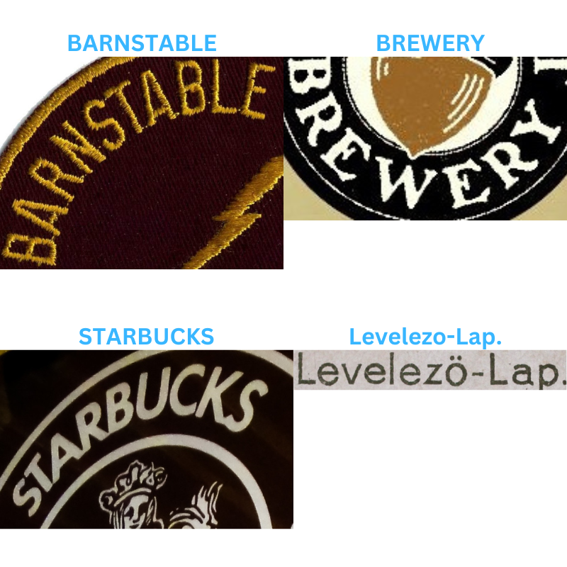
A few things become apparent from the above image. Along with curved text images, the dataset also contains blurry and hazy images. Such real-world image variations pose challenges to deep learning models. Gaining an understanding of the features of images and text in such diverse datasets becomes imperative for state-of-the-art performance of any OCR model. This presents an intriguing challenge for the TrOCR model Naturally, post training, it will perform significantly better on such images.

Fine Tuning TrOCR on Curved Text

Let’s jump into the technical aspects of the article. From here on, we will discuss the code for the TrOCR training process in detail. All the code is available in a Jupyter Notebook through the download link.

Click here to download the source code to this post

Installing and Importing Required Libraries

The first step is to install all the necessary libraries. 

!pip install -q transformers
!pip install -q sentencepiece
!pip install -q jiwer
!pip install -q datasets
!pip install -q evaluate
!pip install -q -U accelerate


!pip install -q matplotlib
!pip install -q protobuf==3.20.1
!pip install -q tensorboard

Among these, some of the important ones are:

• transformers: This is the Hugging Face transformers library that gives us access to hundreds of transformer based models including the TrOCR model.
• sentencepiece: This is the sentencepiece tokenizer library that is needed to convert words into tokens and numbers. This is also part of the Hugging Face family.
• jiwer: The jiwer library gives us access to several speech recognition and language recognition metrics. These include WER (Word Error Rate) and CER (Character Error Rate). We will use the CER metric to evaluate the model while training.

Next, we import all the necessary libraries and packages.

import os
import os
import torch
import evaluate
import numpy as np
import pandas as pd
import glob as glob
import torch.optim as optim
import matplotlib.pyplot as plt
import torchvision.transforms as transforms


from PIL import Image
from zipfile import ZipFile
from tqdm.notebook import tqdm
from dataclasses import dataclass
from torch.utils.data import Dataset
from urllib.request import urlretrieve
from transformers import (
    VisionEncoderDecoderModel,
    TrOCRProcessor,
    Seq2SeqTrainer,
    Seq2SeqTrainingArguments,
    default_data_collator
)

Some of the important import statements from the above code block are:

• VisionEncoderDecoderModel: We need this class to define different TrOCR models.
• TrOCRProcessor: TrOCR expects the dataset to follow a particular normalization process. This class will ensure that the images are properly normalized and processed.
• Seq2SeqTrainer: This is needed to initialize the trainer API.
• Seq2SeqTrainingArguments: While training, the trainer API expects several arguments. The Seq2SeqTrainingArguments class initializes all the required arguments before passing them to the API.
• transforms: The Torchvision transforms module is needed to apply data augmentation to the images.

Now, set the seed for reproducibility across different runs and define the computation device.

def seed_everything(seed_value):
    np.random.seed(seed_value)
    torch.manual_seed(seed_value)
    torch.cuda.manual_seed_all(seed_value)
    torch.backends.cudnn.deterministic = True
    torch.backends.cudnn.benchmark = False

seed_everything(42)

device = torch.device('cuda' if torch.cuda.is_available() else 'cpu')

Download and Extract the Dataset

The next code block contains a helper function to download the CTW1500 data and extract it.

def download_and_unzip(url, save_path):
    print(f"Downloading and extracting assets....", end="")


    # Downloading zip file using urllib package.
    urlretrieve(url, save_path)


    try:
        # Extracting zip file using the zipfile package.
        with ZipFile(save_path) as z:
            # Extract ZIP file contents in the same directory.
            z.extractall(os.path.split(save_path)[0])


        print("Done")


    except Exception as e:
        print("\nInvalid file.", e)


URL = r"https://www.dropbox.com/scl/fi/vyvr7jbdvu8o174mbqgde/scut_data.zip?rlkey=fs8axkpxunwu6if9a2su71kxs&dl=1"
asset_zip_path = os.path.join(os.getcwd(), "scut_data.zip")

# Download if asset ZIP does not exist.
if not os.path.exists(asset_zip_path):
    download_and_unzip(URL, asset_zip_path)

The dataset structure will look like this after extracting the model.

scut_data/
├── scut_train
├── scut_test
├── scut_train.txt
└── scut_test.txt

The data is extracted into the scut_data directory. It contains the scut_train and scut_test subdirectories that hold the training and validation images. 

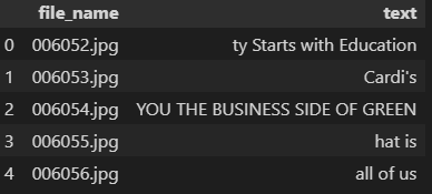
The two text files contain the annotations in the following format.

006052.jpg ty Starts with Education
006053.jpg Cardi's
006054.jpg YOU THE BUSINESS SIDE OF GREEN
006055.jpg hat is
...

Each row contains an image file name and the text in the image is separated by spaces. The number of rows in the text file is the same as the number of samples in the image folders. The text from the image and the image file name are separated by the first space. The image file name must not contain any empty spaces, otherwise, it will be considered part of the text.

Defining Configurations

Before we get to the training part, let’s define the training, dataset, and model configurations.

@dataclass(frozen=True)
class TrainingConfig:
    BATCH_SIZE:    int = 48
    EPOCHS:        int = 35
    LEARNING_RATE: float = 0.00005

@dataclass(frozen=True)
class DatasetConfig:
    DATA_ROOT:     str = 'scut_data'

@dataclass(frozen=True)
class ModelConfig:
    MODEL_NAME: str = 'microsoft/trocr-small-printed'

The model will undergo 35 epochs of training using a batch size of 48.  The learning rate for the optimizer is set at 0.00005. Higher learning rates can make the training process unstable leading to higher loss from the beginning.

Furthermore, we also define the root dataset directory and the model that we are going to use. The TrOCR Small Printed model will be fine-tuned, as it demonstrated optimal performance based on experimentation with this dataset.

A detailed explanation of all the models can be found in the TrOCR inference blog post.

Visualizing a Few Samples

Let’s visualize a few images from the downloaded dataset along with their file names.

def visualize(dataset_path):
    plt.figure(figsize=(15, 3))
    for i in range(15):
        plt.subplot(3, 5, i+1)
        all_images = os.listdir(f"{dataset_path}/scut_train")
        image = plt.imread(f"{dataset_path}/scut_train/{all_images[i]}")
        plt.imshow(image)
        plt.axis('off')
        plt.title(all_images[i].split('.')[0])
    plt.show()


visualize(DatasetConfig.DATA_ROOT)

Preparing the Dataset

The labels are present in text file formats. For smoother data loader preparation, they will need to be modified to an easier format. Let’s convert the training and test text files into Pandas DataFrame.

train_df = pd.read_fwf(
    os.path.join(DatasetConfig.DATA_ROOT, 'scut_train.txt'), header=None
)
train_df.rename(columns={0: 'file_name', 1: 'text'}, inplace=True)
test_df = pd.read_fwf(
    os.path.join(DatasetConfig.DATA_ROOT, 'scut_test.txt'), header=None
)
test_df.rename(columns={0: 'file_name', 1: 'text'}, inplace=True)

Now, the file_name column contains all the file names corresponding to the images and the text column contains the text from the image.

The next step is defining the augmentations.

# Augmentations.
train_transforms = transforms.Compose([
    transforms.ColorJitter(brightness=.5, hue=.3),
    transforms.GaussianBlur(kernel_size=(5, 9), sigma=(0.1, 5)),
])

We apply ColorJitter and GaussianBlur to the images. There is no need to apply any rotation of flipping to the images as there is already enough variability in the original dataset.

The best way to prepare the dataset is to write a custom dataset class. This allows us to have finer control over the inputs. The following code block defines a CustomOCRDataset class to prepare the dataset.

class CustomOCRDataset(Dataset):
    def __init__(self, root_dir, df, processor, max_target_length=128):
        self.root_dir = root_dir
        self.df = df
        self.processor = processor
        self.max_target_length = max_target_length


    def __len__(self):
        return len(self.df)


    def __getitem__(self, idx):
        # The image file name.
        file_name = self.df['file_name'][idx]
        # The text (label).
        text = self.df['text'][idx]
        # Read the image, apply augmentations, and get the transformed pixels.
        image = Image.open(self.root_dir + file_name).convert('RGB')
        image = train_transforms(image)
        pixel_values = self.processor(image, return_tensors='pt').pixel_values
        # Pass the text through the tokenizer and get the labels,
        # i.e. tokenized labels.
        labels = self.processor.tokenizer(
            text,
            padding='max_length',
            max_length=self.max_target_length
        ).input_ids
        # We are using -100 as the padding token.
        labels = [label if label != self.processor.tokenizer.pad_token_id else -100 for label in labels]
        encoding = {"pixel_values": pixel_values.squeeze(), "labels": torch.tensor(labels)}
        return encoding

The __init__() method accepts the root directory path, the DataFrame, TrOCR processor, and the maximum label length as parameters.

The __getitem__() method first reads the label and image from the disk. It then passes the image through the transforms to apply the augmentations. The TrOCRProcessor returns the normalized pixel values in PyTorch tensor format. Next, the text labels are passed through the tokenizer. If a label is shorter than 128 characters, it is padded with -100 to a length of 128. If it is longer than 128 characters, then the characters are truncated.  Finally, it returns the pixel values and the labels as a dictionary.

Before creating the training and validation set, it is necessary to initialize the TrOCRProcessor so that it can be passed to the dataset class.

processor = TrOCRProcessor.from_pretrained(ModelConfig.MODEL_NAME)
train_dataset = CustomOCRDataset(
    root_dir=os.path.join(DatasetConfig.DATA_ROOT, 'scut_train/'),
    df=train_df,
    processor=processor
)
valid_dataset = CustomOCRDataset(
    root_dir=os.path.join(DatasetConfig.DATA_ROOT, 'scut_test/'),
    df=test_df,
    processor=processor
)

This concludes the process of dataset preparation for fine tuning TrOCR model.

Prepare the TrOCR Small Printed Model

The VisionEncoderDecoderModel class gives us access to all the TrOCR models. The from_pretrained() method accepts the repository name to load a pretrained model.

model = VisionEncoderDecoderModel.from_pretrained(ModelConfig.MODEL_NAME)
model.to(device)
print(model)
# Total parameters and trainable parameters.
total_params = sum(p.numel() for p in model.parameters())
print(f"{total_params:,} total parameters.")
total_trainable_params = sum(
    p.numel() for p in model.parameters() if p.requires_grad)
print(f"{total_trainable_params:,} training parameters.")

The model contains 61.5 million parameters. Fine tuning will be done to all the parameters so they can be trained.

One of the most important aspects of model preparation is the model configurations. The configurations are discussed below.

# Set special tokens used for creating the decoder_input_ids from the labels.
model.config.decoder_start_token_id = processor.tokenizer.cls_token_id
model.config.pad_token_id = processor.tokenizer.pad_token_id
# Set Correct vocab size.
model.config.vocab_size = model.config.decoder.vocab_size
model.config.eos_token_id = processor.tokenizer.sep_token_id


model.config.max_length = 64
model.config.early_stopping = True
model.config.no_repeat_ngram_size = 3
model.config.length_penalty = 2.0
model.config.num_beams = 4

The pretrained TrOCR model comes with its own set of predefined configurations. However, to fine tune the model, we will overwrite some of them, which include the token IDs, the vocabulary size, and also the End of Sequence token.

Furthermore, early stopping is set to True. This ensures that if the model metrics do not improve for a few consecutive epochs, then the training will stop.

Optimizer and Evaluation Metric

For optimizing the model weights, we choose the AdamW optimizer with a weight decay of 0.0005.

optimizer = optim.AdamW(
    model.parameters(), lr=TrainingConfig.LEARNING_RATE, weight_decay=0.0005
)

The evaluation metric is going to be CER (Character Error Rate).

cer_metric = evaluate.load('cer')


def compute_cer(pred):
    labels_ids = pred.label_ids
    pred_ids = pred.predictions


    pred_str = processor.batch_decode(pred_ids, skip_special_tokens=True)
    labels_ids[labels_ids == -100] = processor.tokenizer.pad_token_id
    label_str = processor.batch_decode(labels_ids, skip_special_tokens=True)


    cer = cer_metric.compute(predictions=pred_str, references=label_str)


    return {"cer": cer}

Without elaborating further, CER is basically the number of characters that the model did not predict correctly. The lower the CER, the better the performance of the model.

Note that we are skipping the padding token in the calculation of CER as we do not want the padding token to influence the performance of the model.

Training and Validation of TrOCR

The training arguments must be initialized before the training can begin.

training_args = Seq2SeqTrainingArguments(
    predict_with_generate=True,
    evaluation_strategy='epoch',
    per_device_train_batch_size=TrainingConfig.BATCH_SIZE,
    per_device_eval_batch_size=TrainingConfig.BATCH_SIZE,
    fp16=True,
    output_dir='seq2seq_model_printed/',
    logging_strategy='epoch',
    save_strategy='epoch',
    save_total_limit=5,
    report_to='tensorboard',
    num_train_epochs=TrainingConfig.EPOCHS
)

The FP16 training is being used as it uses less GPU memory and also allows us to use a higher batch size. Also, the logging and model-saving strategy is based on epochs. All the reports will be logged to tensorboard.

These training arguments will be passed to the trainer API along with the other required arguments.

# Initialize trainer.
trainer = Seq2SeqTrainer(
    model=model,
    tokenizer=processor.feature_extractor,
    args=training_args,
    compute_metrics=compute_cer,
    train_dataset=train_dataset,
    eval_dataset=valid_dataset,
    data_collator=default_data_collator
)

The training process can be commenced by calling the train() method of the trainer object.

res = trainer.train()

Epoch Training Loss Validation Loss Cer
1 3.822000 2.677871 0.687739
2 2.497100 2.474666 0.690800
3 2.180700 2.336284 0.627641
.
.
.
33 0.146800 2.130022 0.504209
34 0.145800 2.167060 0.511095
35 0.138300 2.120335 0.494496

By the end of training, the model reaches a CER of 49% which is a very good result considering the small TrOCR model used.

Following is the CER graph from the Tensorboard logs.

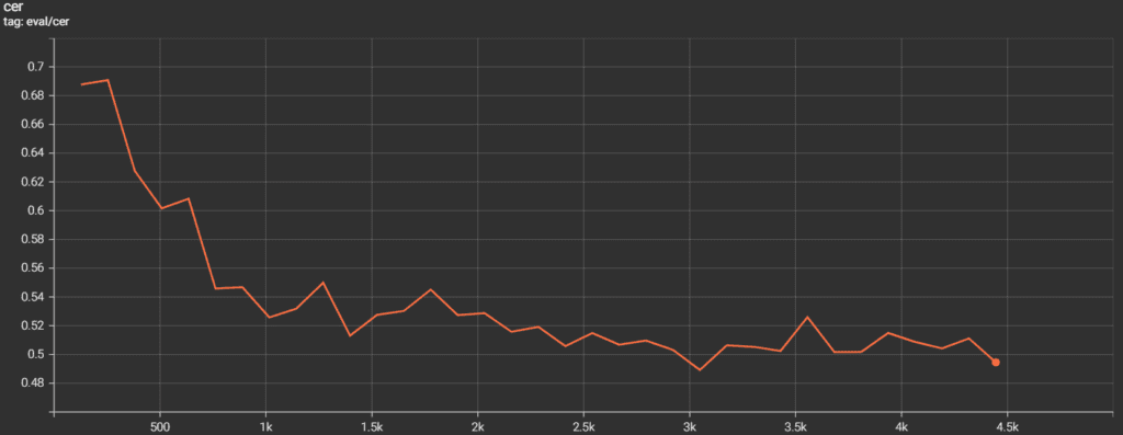
The curve is on a decreasing trend till the end of training. Although training for longer may give better results, we will continue using the model we have.

Inference using the Fine Tuned TrOCR Model

Having trained the TrOCR model, it’s time to run inferences on the validation images.

The first step is to load the trained model from the last saved checkpoint.

processor = TrOCRProcessor.from_pretrained(ModelConfig.MODEL_NAME)
trained_model = VisionEncoderDecoderModel.from_pretrained('seq2seq_model_printed/checkpoint-'+str(res.global_step)).to(device)

The res object contains a global_step attribute that holds the total number of steps the model was trained for. The above code block uses that attribute to load the weights from the final epoch.

Up next are some helper functions. The first one is to read an image.

def read_and_show(image_path):
    """
    :param image_path: String, path to the input image.


    Returns:
        image: PIL Image.
    """
    image = Image.open(image_path).convert('RGB')
    return image

The next helper function carries out the forward pass of the image through the model.

def ocr(image, processor, model):
    """
    :param image: PIL Image.
    :param processor: Huggingface OCR processor.
    :param model: Huggingface OCR model.


    Returns:
        generated_text: the OCR'd text string.
    """
    # We can directly perform OCR on cropped images.
    pixel_values = processor(image, return_tensors='pt').pixel_values.to(device)
    generated_ids = model.generate(pixel_values)
    generated_text = processor.batch_decode(generated_ids, skip_special_tokens=True)[0]
    return generated_text

The final helper function loops over all the images in a directory and keeps on calling the ocr() function for inference.

def eval_new_data(
    data_path=os.path.join(DatasetConfig.DATA_ROOT, 'scut_test', '*'),
    num_samples=50
):
    image_paths = glob.glob(data_path)
    for i, image_path in tqdm(enumerate(image_paths), total=len(image_paths)):
        if i == num_samples:
            break
        image = read_and_show(image_path)
        text = ocr(image, processor, trained_model)
        plt.figure(figsize=(7, 4))
        plt.imshow(image)
        plt.title(text)
        plt.axis('off')
        plt.show()

eval_new_data(
    data_path=os.path.join(DatasetConfig.DATA_ROOT, 'scut_test', '*'),
    num_samples=100
)

We are running inference on 100 samples (num_samples=100).

Here are two results that the model was OCRing wrongly before training.

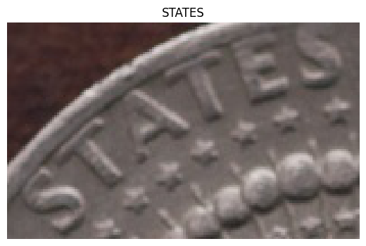
The results are impressive. After fine tuning the TrOCR model, it is able to predict the text in curved and vertical images correctly. 

Here are some more results where the model performs well.

In this case, although the text at the extreme ends is stretched, still the model predicts them correctly.

Figure 9. TrOCR inference results on blurry text.

In the above three cases, the model predicts the text correctly even though they are blurry.

Conclusion

In this article, we went through the fine tuning of the TrOCR model on a curved text recognition dataset. We started with the dataset discussion. This was followed by dataset preparation and training of the TrOCR model. After training, we ran inference experiments and analyzed the results. Our results indicated that fine tuning the TrOCR model can result in better performance, even on blurry or curved text images.

OCR is not just about recognizing text in a scene, it is also about building applications using OCR, like a Captcha recognizer or combining the TrOCR recognizer with a license plate detection pipeline.

Let us know in the comments what interesting applications you are thinking of building with TrOCR.