Fine-tuning BERT can help expand its language understanding capability to newer domains of text. What sets BERT apart is its ability to grasp the contextual relationships of a sentence, understanding the meaning of each word in relation to its neighbor. In continuation of our previous article, we will be training BERT using Hugging Face Transformers and also will teach BERT to analyze abstracts from Arxiv and classify them into one of 11 categories.

What’s the agenda of this blog post?
- We will start with installing the dependencies.
- Then we will move on to the explanation of the dataset that we will use for fine-tuning BERT.
- This will be followed by preparing the model and training.
- To wrap up, we will run inference on unseen abstracts to test the fine-tuned BERT model.
Why Fine-Tuning BERT Matters?
While the pre-trained BERT model is powerful, it’s a generalized tool. It understands language but isn’t tailored for any specific task. Fine-tuning, in essence, is the act of adapting this generalized tool for a specialized job.
Hugging Face Transformers
Hugging Face Transformers is a library that’s become synonymous with state-of-the-art NLP. With its user-friendly interface and extensive model repository, Hugging Face makes it straightforward to fine-tune models like BERT. For our task, we’ll be leveraging this library, ensuring the process is both smooth and efficient.
Should you require a recap, consider revisiting our previous post on Hugging Face Transformers for BERT NLP tasks.
Fine-Tuning BERT on the Arxiv Abstract Classification Dataset
For fine-tuning BERT, first, we need to install some dependencies.
!pip install -U transformers datasets evaluate accelerate
!pip install scikit-learn
!pip install tensorboard
The Hugging Face transformers library provides us with pre-trained NLP models (like BERT) and utilities for fine-tuning and deploying them. Alongside it, the datasets library from Hugging Face offers a plethora of datasets.
evaluate is a utility that provides evaluation metrics, and accelerate is a library by Hugging Face designed to abstract away the complexities of launching training on hardware accelerators (like GPUs or TPUs).
We also need the Scikit-Learn library for creating the training and validation splits and TensorBoard for logging.
Importing the Necessary Libraries
The next step is importing the necessary libraries, modules, and packages.
from datasets import load_dataset
from transformers import (
    AutoTokenizer,
    DataCollatorWithPadding,
    AutoModelForSequenceClassification,
    TrainingArguments,
    Trainer,
    pipeline,
)

import evaluate
import glob
import numpy as np
Let’s go through the explanation of the important ones.
AutoTokenizer: This aids in tokenizing our text data into a format BERT can understand. The “Auto” prefix means it can infer the appropriate tokenizer for various models.
DataCollatorWithPadding: Ensures that our tokenized data is batched together with consistent lengths, adding padding where necessary. It’s crucial for training stability and efficiency.
AutoModelForSequenceClassification: A generic class that can instantiate model architectures tailored for sequence classification tasks. Again, the “Auto” prefix makes it versatile across various pre-trained models.
TrainingArguments: A convenient way to define the training configuration, such as the learning rate, batch size, and number of epochs.
Trainer: A high-level utility from the Transformers library that abstracts the training and evaluation loop, making fine-tuning straightforward.
Pipeline: Simplifies the process of applying models on data. It’s a handy tool for post-training evaluations and predictions.
Setting the Hyperparameters for Fine-Tuning BERT
Training hyperparameters are an important part of any deep learning training pipeline. To get the best possible results while fine-tuning BERT, we need to choose the hyperparameters wisely.
BATCH_SIZE = 32
NUM_PROCS = 32
LR = 0.00005
EPOCHS = 5
MODEL = 'bert-base-uncased'
OUT_DIR = 'arxiv_bert'
We set both batch size and number of parallel processes as 32. The fine-tuning notebook provided was run on a machine with RTX A5000 GPU and Ryzen processor. So, you can decrease or increase the above two according to your system configuration.
The base learning rate is set at 0.00005 marking it as a vital hyperparameter. A smaller value, like 0.00005, ensures that the model trains slower and is precise, avoiding overshooting the minimum. However, it might also mean longer training times.
The model will be trained for 5 epochs.
The model is ‘bert-base-uncased’ and is a version of BERT that’s trained on lowercase English text (hence ‘uncased’). It is one of the smaller variants of BERT, making it faster to train while still being powerful.
The OUT_DIR indicates the directory location where all the logs and models will be saved.
Download and Prepare the Dataset
Dataset preparation is one of the most important tasks. However, Hugging Face makes dataset related tasks a lot simpler. The following code will make things even simpler.
train_dataset = load_dataset("ccdv/arxiv-classification", split='train')
valid_dataset = load_dataset("ccdv/arxiv-classification", split='validation')
test_dataset = load_dataset("ccdv/arxiv-classification", split='test')
print(train_dataset)
print(valid_dataset)
print(test_dataset)
We’re utilizing the load_dataset function from the Hugging Face datasets library to fetch the arxiv-classification dataset from its hub. The split argument allows us to load specific portions of this dataset:
train: This is the main bulk of the dataset and will be used to train our model.
validation: A subset of the data that the model hasn’t seen during training.
test: This portion is reserved for the final evaluation. It gives us an unbiased evaluation of the model’s performance.
Printing the datasets gives the following output.
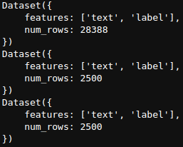
As we can see there are around 28000 training samples, 2500 validation samples, and 2500 test samples.
Let’s visualize one of the samples from the training set.
# Visualize a sample.
train_dataset[0]
{'text': 'Constrained Submodular Maximization via a\nNon-symmetric Technique\n\narXiv:1611.03253v1 [cs.DS] 10 Nov 2016\n\nNiv Buchbinder∗\n\nMoran Feldman†\n\nNovember 11, 2016\n\nAbstract\nThe
.
.
.
'label': 8}
It contains the ‘text’ key and the ‘label’ key. The former contains the abstract text and the latter the label number.
Dataset Label Information
Currently, we’re familiar with the label numbers. By mapping the label names to these IDs, we can get a clearer picture of the dataset.
id2label = {
    0: "math.AC",
    1: "cs.CV",
    2: "cs.AI",
    3: "cs.SY",
    4: "math.GR",
    5: "cs.CE",
    6: "cs.PL",
    7: "cs.IT",
    8: "cs.DS",
    9: "cs.NE",
    10: "math.ST"
}
label2id = {
    "math.AC": 0,
    "cs.CV": 1,
    "cs.AI": 2,
    "cs.SY": 3,
    "math.GR": 4,
    "cs.CE": 5,
    "cs.PL": 6,
    "cs.IT": 7,
    "cs.DS": 8,
    "cs.NE": 9,
    "math.ST": 10
}
The id2label dictionary maps numerical identifiers to their corresponding class names. This is beneficial for two main reasons. label2id is the inverse of the id2label dictionary. It maps class names to their respective numerical identifiers.
Tokenizing the Dataset
Before fine-tuning BERT, our dataset’s text data must be converted into a format the model understands. This process is called tokenization. Let’s break down this essential preprocessing step.
tokenizer = AutoTokenizer.from_pretrained(MODEL)
Using the AutoTokenizer class, we initialize a tokenizer specific to our chosen pre-trained model (bert-base-uncased). This tokenizer knows the vocabulary of the pre-trained model and its special tokens.
def preprocess_function(examples):
    return tokenizer(
        examples["text"],
        truncation=True,
    )
This function is designed to tokenize a batch of textual data. The truncation=True argument ensures that if a text exceeds the model’s max input length, it’s truncated to fit.
We also need to map the processing function to the datasets and apply the preprocessing steps.
tokenized_train = train_dataset.map(
    preprocess_function,
    batched=True,
    batch_size=BATCH_SIZE,
    num_proc=NUM_PROCS
)

tokenized_valid = valid_dataset.map(
    preprocess_function,
    batched=True,
    batch_size=BATCH_SIZE,
    num_proc=NUM_PROCS
)

tokenized_test = test_dataset.map(
    preprocess_function,
    batched=True,
    batch_size=BATCH_SIZE,
    num_proc=NUM_PROCS
)
This may take some time depending on the processing power and cores used in the CPU.
data_collator = DataCollatorWithPadding(tokenizer=tokenizer)
When feeding batches of sentences into a model, it’s crucial that all sentences in a batch have the same length. As real-world sentences vary in length, we pad shorter sentences with a special padding token. DataCollatorWithPadding ensures this happens automatically during training. By feeding it, our tokenizer, knows the appropriate padding token and max length to use.
Sample Tokenization Example
Let’s take a look at a simple tokenized input.
tokenized_sample = preprocess_function(train_dataset[0])
print(tokenized_sample)
print(f"Length of tokenized IDs: {len(tokenized_sample.input_ids)}")
print(f"Length of attention mask: {len(tokenized_sample.attention_mask)}")
Taking a Look Tokenized Sample
To understand the tokenization process more concretely, we’re examining the result of tokenizing a single example from our train_dataset. Let’s break down the process and observe the outputs:
tokenized_sample = preprocess_function(train_dataset[0])
print(tokenized_sample)
We tokenize a sample and print it.
The tokenizer returns a dictionary with two key-value pairs: input_ids and attention_mask.
- input_ids: These are the numerical identifiers for each token in the text. For example, the ID 101 corresponds to the special [CLS] token, which BERT uses to indicate the beginning of a sequence.
- attention_mask: This mask identifies which tokens are padding and which aren’t. The model should attend to tokens with a value of 1, while a value of 0 indicates padding tokens. This mask helps the model differentiate between real tokens and padding.
Evaluation Metrics
We will evaluate the accuracy metric using the validation dataset. For that, we need to define a function using the evaluate library.
accuracy = evaluate.load('accuracy')
def compute_metrics(eval_pred):
    predictions, labels = eval_pred
    predictions = np.argmax(predictions, axis=1)
    return accuracy.compute(predictions=predictions, references=labels)
Preparing the BERT Model
The ultimate objective is fine-tuning a pre-trained BERT model on our specific classification task. Here, we are initializing a model tailored for sequence classification tasks:
model = AutoModelForSequenceClassification.from_pretrained(
    MODEL,
    num_labels=11,
    id2label=id2label,
    label2id=label2id,
)
The above code initializes the BERT model from the AutoModelForSequenceClassification class. As per our dataset, the number of classes are 11. The id mappings will provide a more comprehensive output during inference.
The final BERT model has 109 million parameters.
Training Arguments
Before starting the training, the arguments need to be defined.
training_args = TrainingArguments(
    output_dir=OUT_DIR,
    learning_rate=LR,
    per_device_train_batch_size=BATCH_SIZE,
    per_device_eval_batch_size=BATCH_SIZE,
    num_train_epochs=EPOCHS,
    weight_decay=0.01,
    evaluation_strategy="epoch",
    save_strategy="epoch",
    load_best_model_at_end=True,
    save_total_limit=3,
    report_to='tensorboard',
    fp16=True
)
Let’s look at some of the important training hyperparameters:
- learning_rate: The learning rate for the optimizer. A smaller learning rate implies slower convergence but potentially better generalization.
- per_device_train_batch_size & per_device_eval_batch_size: Batch size during training and evaluation. This determines how many samples are processed at once.
- num_train_epochs: The total number of times the training set will be iterated over.
- weight_decay: Regularization technique to prevent overfitting. It adds a penalty to the magnitude of the model parameters.
The following are the evaluation parameters.
- evaluation_strategy: This means evaluation will be performed at the end of each epoch.
- save_strategy: The model will be saved at the end of each epoch.
- load_best_model_at_end: After all training epochs, the model with the best evaluation metric will be reloaded.
- save_total_limit: This limits the number of model checkpoints that are saved. Only the last 3 checkpoints will be kept, helping in managing storage.
Finally, everything will be logged to TensorBoard, and FP16 precision will be used for training.
Initializing the Trainer
Finally, we are all set to initialize the trainer and start the training process.
trainer = Trainer(
    model=model,
    args=training_args,
    train_dataset=tokenized_train,
    eval_dataset=tokenized_valid,
    tokenizer=tokenizer,
    data_collator=data_collator,
    compute_metrics=compute_metrics,
)

history = trainer.train()
Following are the output logs from the training.
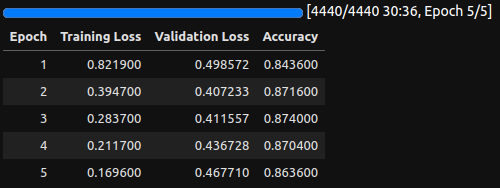
The model reaches an accuracy of more than 86% in just 5 epochs.

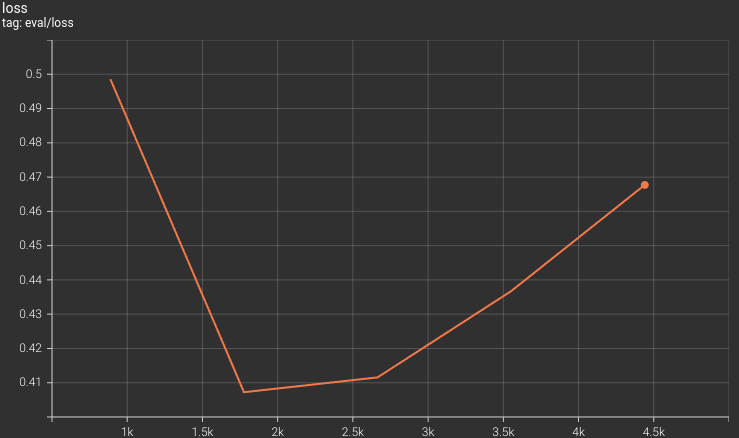
Taking a look at the accuracy and loss plots reveal that the final model may be slightly overfit. Using a learning rate scheduler in this case will surely help.
Evaluation
We can use the best model for evaluation on the test set.
trainer.evaluate(tokenized_test)
{'eval_loss': 0.38107171654701233,
'eval_accuracy': 0.8796,
'eval_runtime': 14.9454,
'eval_samples_per_second': 167.276,
'eval_steps_per_second': 2.676,
'epoch': 5.0}
Our model is achieving almost 88% accuracy on the test set.
Inference on Unseen Data
For the final experiments, we will pass a few unseen abstracts from Arxiv through our model and see how it performs. These abstracts are present in the inference_data directory in separate text files. The name of the text files represents the ground truth label.
AutoModelForSequenceClassification.from_pretrained(f"arxiv_bert/checkpoint-4440")

tokenizer = AutoTokenizer.from_pretrained('bert-base-uncased')
classify = pipeline(task='text-classification', model=model, tokenizer=tokenizer)

all_files = glob.glob('inference_data/*')
for file_name in all_files:
    file = open(file_name)
    content = file.read()
    print(content)
    result = classify(content)
    print('PRED: ', result)
    print('GT: ', file_name.split('_')[-1].split('.txt')[0])
    print('\n')
The final model is loaded from the disk, the tokenizer is initialized, and the classification pipeline is loaded.
We loop over each text file, and forward pass them through the model to obtain the results.
Taking a look at the results reveals that the model makes just one mistake where it predicts a CS.CV label as CS.NE. It gets all other 9 predictions right which is impressive for just 5 epochs of training.
Summary and Conclusion
Leveraging the Hugging Face Transformers library, this article covered the intricate process of fine-tuning BERT for classifying arxiv abstracts into one of 11 distinct categories. From initial setups, importing necessary libraries, and setting hyperparameters, to the crux of data tokenization and model training, each step was demystified.
This opens many avenues for AI enthusiasts like you to fine-tune BERT on many real-world datasets and build applications. Starting from sentiment analysis to rating restaurant reviews, a lot of processes can be automated.
Let us know in the comments what you are going to build using BERT.









100K+ Learners
Join Free OpenCV Bootcamp3 Hours of Learning