Face Recognition with ArcFace

Can we distinguish one person from another by looking at the face? We can probably list several features such as eye color, hairstyle, skin tone, the shape of the nose and eyebrows, etc. Some combination of such attributes will be unique to a particular person. Sometimes, people have visual similarities, and in rare cases, it becomes difficult to distinguish one from another.

Can we program computers to do this task automatically? Suppose you enumerate all these features which describe personality and try to build a decision tree in an if-else manner pretty quickly. In that case, there will be a combinatorial explosion of various choices. So, we need a more general representation instead of a list of specific features.

The post is divided into the following sub-topics:

1. Feature Extraction with Deep Neural Network
2. Background of Face Recognition
3. Introduction to ArcFace and Comparison with Softmax Loss
4. Metric for Computing Embedding Pair Score
5. Performing Inference with ArcFace Model
   1. Different People
   2. Pose Variation
   3. Corner Cases
6. Visualizing embeddings with tSNE

During the classical machine learning era, researchers in the computer vision field came up with various ideas on extracting representation from images. For example, using some combinations of traditional feature extractors and descriptors. Fortunately, deep neural networks have the ability to learn such representation from data automatically.

Many practical tasks can be solved by learning good representation. If you look at other machine learning areas, such as Natural Language Processing and Recommendation Systems, you may notice another name for this – embeddings.

Embedding is a vector of real numbers which contains all extracted information. It is assumed that embeddings for semantically similar objects are close in terms of some metric. So, if you have good embeddings, you can compare them with each other or search for the closest. For example, you can learn embeddings for movies and recommend the top-5 most similar ones to the user based on their liking. Also, they have some interesting properties. As noted by the authors of the famous word2vec family of models for word embeddings, arithmetic operations can be applied to them.

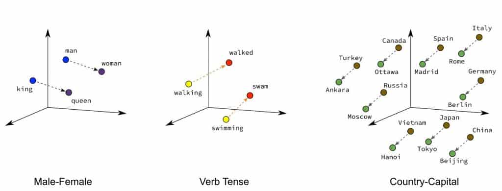
Nowadays, embeddings have become an integral part of solutions to many problems. Facial recognition is using the same approach. Usually supposed, the similarity of a pair of faces can be directly calculated by computing their embeddings’ similarity. In this case, the face recognition task is trivial: we only need to check if the distance between the two vectors exceeds a predefined threshold. So, our main goal is to understand how to train a model capable of extracting appropriate embeddings from faces.

Feature Extraction – Face Recognition with Arcface

Deep Neural Networks have widespread use in computer vision as feature extractors. Certain ideas and mechanisms like stacking layers, skip-connections, SE-blocks, etc., subsequently became an essential part of any contemporary deep learning architecture, but the main principle is the same. There is a backbone with convolution layers and some head which uses extracted information to solve the specific task (usually head is fully connected to layers like in simple classification cases). So, the forward pass should sound familiar.

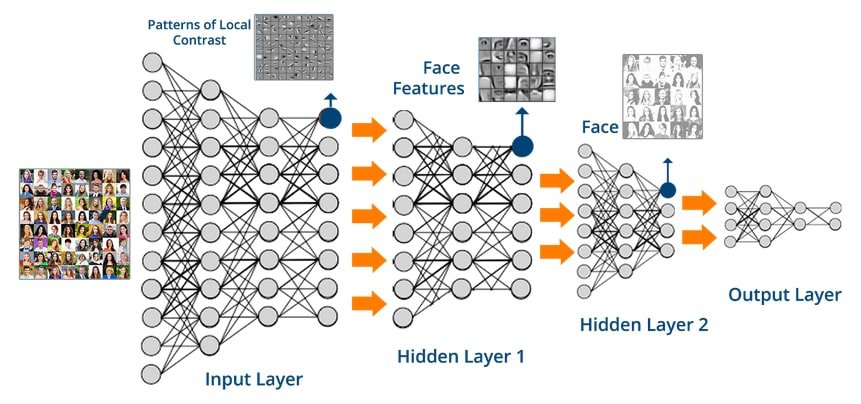
To train neural networks, we need a loss function for which gradients are calculated during the backward pass, and then model weights are updated with some optimizer. For image classification tasks, cross-entropy loss (some people call softmax loss) is usually used. And now, the tricky part begins. How suitable is such a loss for embedding training? Can we think of something better? Or we need to drastically change the training technique for our face recognition model? To answer these questions, let’s review what machine learning practitioners have come up with within the last few years to solve this problem.

Background of Face Recognition

In our case, Neural Network is a complex mapping function from the image to the vector space. The goal is to distinguish in this vector space identity of one person from another. The intra-class compactness and inter-class separability are important factors in feature discrimination ability. Embeddings belonging to the same identity are expected to be closer in the representation space, while embeddings of different identities are expected to be scattered. Several loss functions have been designed to get this property from embeddings during the training procedure.

In previous years, the similarity learning approach used to be quite popular. The first example of this type is the Siamese Network with contrastive loss. This paper was published in 2005 under the supervision of Yann LeCun, one of the most influential researchers in the deep learning field. Another example is FaceNet with triplet loss. Both the contrastive loss and triplet losses penalize the distance between two embeddings, such that the similarity metric will be small for pairs of faces from the same person and large for pairs from different people. It is worth noting that both losses require a carefully designed pair selection, which is the obvious disadvantage. More novel approaches have been proposed in the last couple of years.

Another type of loss uses the angular margin penalty to enforce intra-class compactness and inter-class difference of embeddings on the hypersphere surface. SphereFace introduced the important idea of angular margin in 2017. A year later, an improvement was suggested in CosFace with a cosine margin penalty. At the same time, ArcFace was developed on similar principles. Let’s take a closer look and understand this state-of-the-art method which has received fairly widespread adoption.

ArcFace Loss

Besides the backbone that extracts features, there is the head for classification with a fully connected layer with trainable weights. The product of normalized weights and normalized features lie in the interval from -1 to 1. We can represent a logit for each class as the cosine of an angle between the feature and the ground truth weight inside a hypersphere with a unit radius. Also, there are two hyperparameters m (the additional angular margin) and s (scaling ratio from a small number to a final logit), that help adjust the distance between classes.

To illustrate the geometric intuition behind those formulas, the authors trained their model to discriminate between 8 identities for 2D embeddings both with softmax and ArcFace loss. The learned embeddings are distributed on a hypersphere (in 2D it is just a circle) with a radius of s. You can notice that each identity has a separate color and a center around which the points are distributed.

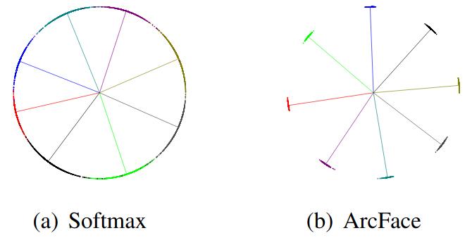
With softmax loss embeddings can be roughly separated, there is uncertainty where decision boundaries can be placed. In practice, this means that faces that look similar will be tough to distinguish.

Another issue with using pure softmax loss is, that number of weights in the last fully connected layer increases linearly with the number of classes. So, it is quite problematic to train a neural network capable of distinguishing between millions of personalities.

ArcFace loss does not have this shortage, and the result seems much better. All points are closer to the center, and there is an evident gap between identities. Consequently, the previously mentioned requirements for intra-class compactness and inter-class separability are met.

Cosine Distance

To measure the similarity between two embeddings extracted from images of the faces, we need some metrics. Cosine distance is a way to measure the similarity between two vectors, taking a value from 0 to 1. Actually, this metric reflects the orientation of vectors indifferently to their magnitude. If cosine distance is near 0, then vectors have similar orientations and are close to each other. If it is almost 1, then vectors differ (in other words, they are orthogonal).

Here is an example of how we can calculate such a metric in numpy.

from numpy import dot, sqrt

def cosine_similarity(x, y):
    return dot(x, y) / (sqrt(dot(x, x)) * sqrt(dot(y, y)))

If you are interested in a more rigorous mathematical definition or want to refresh your linear algebra knowledge, you can read a wiki article about it.

Inferencing with ArcFace Model

Besides the identification model, face recognition systems usually have other preprocessing steps in a pipeline. Let’s briefly describe them.

First, a face detector must be used to detect a face on an image. After that, we can use face alignment for cases that do not satisfy our model’s expected input. Identification is considered a rather challenging problem, so face alignment is utilized to make the model’s life easier. If a face is transformed into a canonical pose (like the tip of the nose in the center of the image, etc.), the model can focus on getting important information straight away. Finally, we need to crop and resize the face to a specific size (in our examples, it will be 112×112). In real-world scenarios, an additional anti-spoofing model can be used to avoid deception at the identification step, but we’ll leave it behind the scenes.

It is time to take the pre-trained face identification model and check how it works on various examples.

Weights for an ArcFace model and some part of the code have been taken from https://github.com/ZhaoJ9014/face.evoLVe.PyTorch. Thanks to them for sharing!

Different people

Okay, let’s start with two famous actors: Jeff Bridges and Kurt Russell. These guys have some similarities, don’t they?

To evaluate our model, we need to extract embeddings via the backbone from preprocessed images, normalize them, and calculate cosine distance for all pairs.

Click here to download the source code to this post

def visualize_similarity(tag, input_size=[112, 112]):
    images, embeddings = get_embeddings(
        data_root=f"data/{tag}_aligned",
        model_root="checkpoint/backbone_ir50_ms1m_epoch120.pth",
        input_size=input_size,
    )

    # calculate cosine similarity matrix
    cos_similarity = np.dot(embeddings, embeddings.T)
    cos_similarity = cos_similarity.clip(min=0, max=1)
    # plot grid from pair distance values in similarity matrix
    similarity_grid = plot_similarity_grid(cos_similarity, input_size)

    # pad similarity grid with images of faces
    horizontal_grid = np.hstack(images)
    vertical_grid = np.vstack(images)
    zeros = np.zeros((*input_size, 3))
    vertical_grid = np.vstack((zeros, vertical_grid))
    result = np.vstack((horizontal_grid, similarity_grid))
    result = np.hstack((vertical_grid, result))

    if not os.path.isdir("images"):
        os.mkdir("images")

    cv2.imwrite(f"images/{tag}.jpg", result)

Through using this helper function, we will receive a final result in one table.

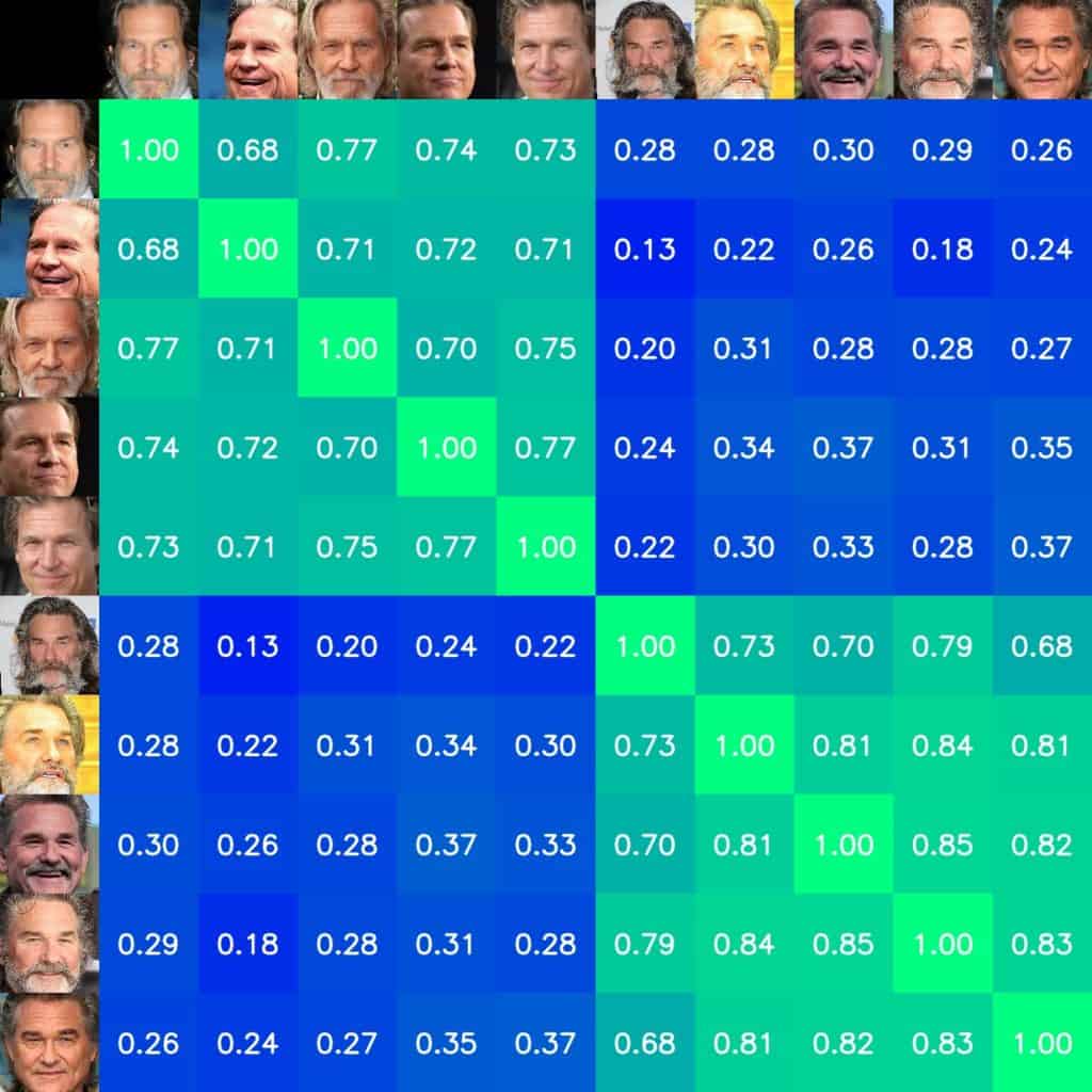
Hmm, not bad! It gives us insight that the predefined threshold can be adjusted to be something like 0.65 or 0.70. In a real use case, such a threshold depends on our risk acceptance and what type of errors we want to minimize, several false positives or false negatives.

Now, let’s try to find similarities between different actresses.

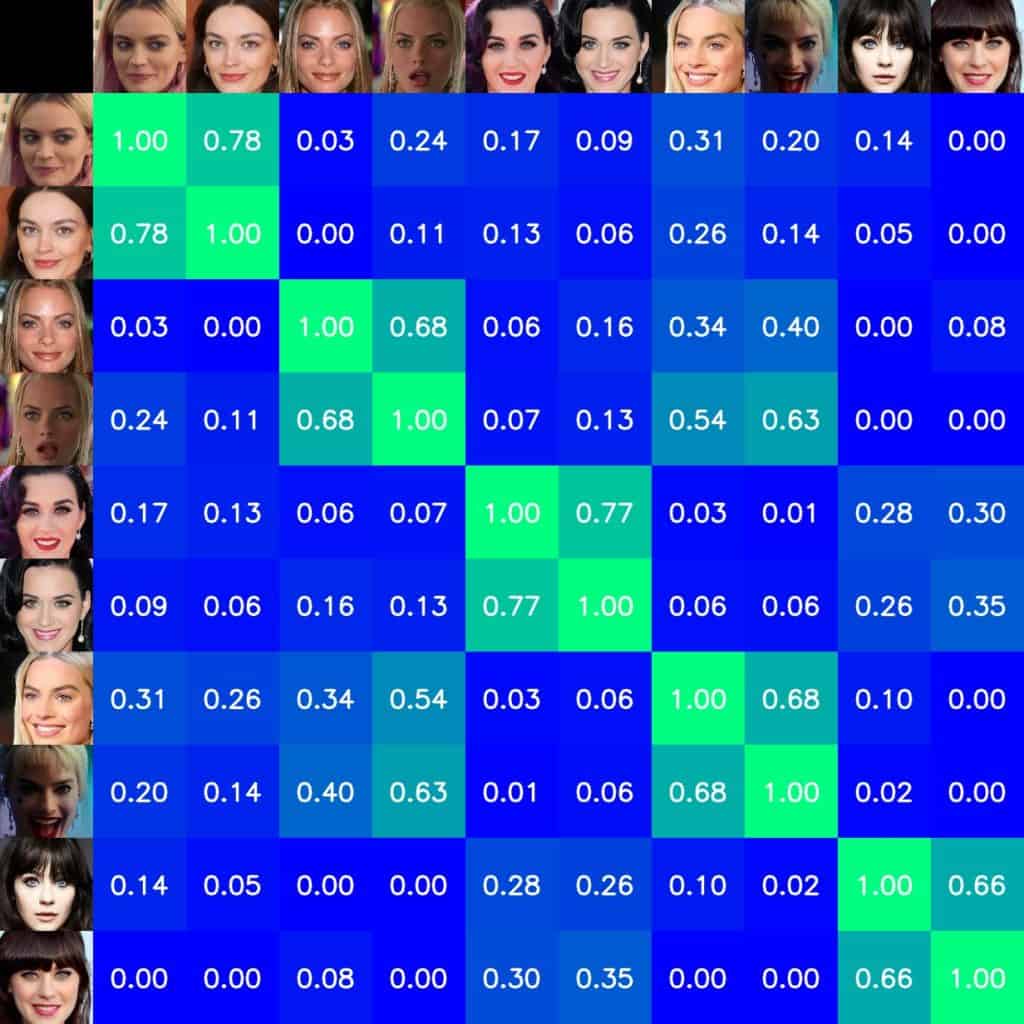
If you look closely, there are patterns in our table. Margot Robbie and Jaime Pressly have a high value of cosine distance and have a similar appearance! Zooey Deschanel and Katy Perry are more similar to each other than to other actresses in this set. So, cosine distance between embeddings reflects our concept of the similarity between people in real life.

The same person in various poses

Now, let’s see how it works with three different head poses.

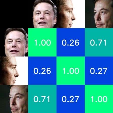
The result of the profile image is rather bad. But with the slightly turned face, it seems to work fine. It can be concluded that our model is susceptible to head rotation.

Corner cases

To avoid falling into the illusion that our model is working in all possible circumstances, let’s try images with various accessories, occlusions, and emotional expressions.

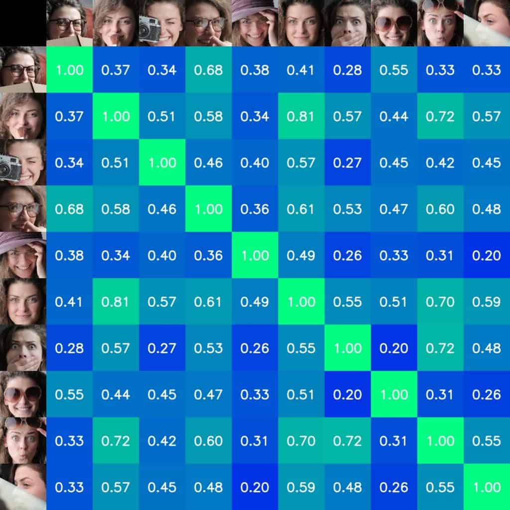
As expected, such corner cases can be too hard for our model. This indicates that models for real-world production face recognition systems must be trained on more diverse data to circumvent such limitations.

t-SNE

To better understand how embeddings are distributed in space, we can use dimensionality reduction algorithms such as t-SNE. If you aren’t familiar with this method, please, read our tsne for feature utilization article.

After applying t-SNE, we will receive a vector with two components instead of 512, and we can easily plot our results on a 2D plane. We will take each coordinate as a center and add an appropriate original face image.

As a result, clusters not only have intra-class compactness and inter-class separability as expected from ArcFace embeddings but also match our intuition about the similarity between these people.

Summary

In this post, we looked at the current state of the face recognition task. We learned that good representation in the form of embeddings is key to solving this problem. Several approaches for training such embeddings have been mentioned, including ArcFace, one of the most important at the moment. Also, we looked at several examples to see how it works (even more important, when it does not work) in practice. Now you can use this knowledge for your own applications!

Must Read Articles