In this tutorial, we will learn about Exposure Fusion using OpenCV. We will share code in C++ and Python.
What is Exposure Fusion?
If you are not aware of HDR imaging or would like to know more, check out our post on HDR imaging using OpenCV.
When we capture a photo using a camera, it has only 8-bits per color channel to represent the brightness of the scene. However, the brightness of the world around us can theoretically vary from 0 ( pitch black ) to almost infinite ( looking straight at the Sun ). So, a point-and-shoot or a mobile camera decides an exposure setting based on the scene so that the dynamic range ( 0-255 values ) of the camera is used to represent the most interesting parts of an image. For example, in many cameras face detection is used to find faces and exposure is set so that the face appears nicely lit.
This begs the question — Can we take multiple pictures at different exposure settings and capture a larger range of brightness of the scene? The answer is a big YES! The traditional way of doing it using HDR imaging followed by tone mapping.
HDR imaging requires us to know the precise exposure time. The HDR image itself looks dark and is not pretty to look at. The minimum intensity in an HDR image is 0, but theoretically, there is no maximum. So we need to map its values between 0 and 255 so we can display it. This process of mapping an HDR image to a regular 8-bit per channel color image is called Tone Mapping.
As you can see, assembling an HDR image and then tone mapping is bit of a hassle. What can’t we just use the multiple images and create a tone mapped image without ever going to HDR. Turns out we can do that using Exposure Fusion.
How does Exposure Fusion work?
The steps for applying exposure fusion are described below
Step 1: Capture multiple images with different exposures
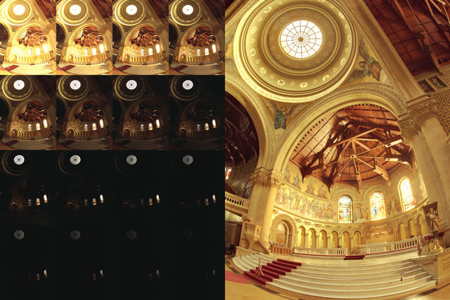
First, we need to capture a sequence of images of the same scene without moving the camera. The images in the sequence have varying exposure as shown above. This is achieved by changing the shutter speed of the camera. Usually, we choose some images that are underexposed, some that are overexposed, and one that it correctly exposed.
In a “correctly” exposed image, the shutter speed is chosen ( either automatically by the camera or by the photographer ) so that the 8-bit per channel dynamic range is used to represent the most interesting parts of the image. The regions that are too dark are clipped to 0 and the regions that are too bright saturate to 255.
In an underexposed image, the shutter speed is fast, and the image is dark. Thus, the 8-bits of the image are used to capture bright areas while the dark regions are clipped to 0.
In an overexposed image, the shutter speed is slow, and so more light is captured by the sensor and therefore the image is bright. The 8-bits of the sensor are used to capture the intensity of dark regions while bright regions saturate to a value of 255.
Most SLR cameras have a feature called Auto Exposure Bracketing (AEB) that allows us to take multiple pictures at different exposures with just one press of a button. If you are using an iPhone, you can use this AutoBracket HDR app and if you are an android user you can try A Better Camera app.
Once we have captured these images, we can use the code below to read them in.
C++
void readImages(vector<Mat> &images)
{

  int numImages = 16;
  static const char* filenames[] =
  {
    "images/memorial0061.jpg",
    "images/memorial0062.jpg",
    "images/memorial0063.jpg",
    "images/memorial0064.jpg",
    "images/memorial0065.jpg",
    "images/memorial0066.jpg",
    "images/memorial0067.jpg",
    "images/memorial0068.jpg",
    "images/memorial0069.jpg",
    "images/memorial0070.jpg",
    "images/memorial0071.jpg",
    "images/memorial0072.jpg",
    "images/memorial0073.jpg",
    "images/memorial0074.jpg",
    "images/memorial0075.jpg",
    "images/memorial0076.jpg"
  };

  for(int i=0; i < numImages; i++)
  {
    Mat im = imread(filenames[i]);
    images.push_back(im);
  }

}
Python
def readImagesAndTimes():

  filenames = [
               "images/memorial0061.jpg",
               "images/memorial0062.jpg",
               "images/memorial0063.jpg",
               "images/memorial0064.jpg",
               "images/memorial0065.jpg",
               "images/memorial0066.jpg",
               "images/memorial0067.jpg",
               "images/memorial0068.jpg",
               "images/memorial0069.jpg",
               "images/memorial0070.jpg",
               "images/memorial0071.jpg",
               "images/memorial0072.jpg",
               "images/memorial0073.jpg",
               "images/memorial0074.jpg",
               "images/memorial0075.jpg",
               "images/memorial0076.jpg"
               ]

  images = []
  for filename in filenames:
    im = cv2.imread(filename)
    images.append(im)

  return images
Step 2: Align Images
The images in the sequence need to be aligned even if they were acquired using a Tripod because even minor camera shake can lower the quality of the final image. OpenCV provides an easy way to align these images using AlignMTB. This algorithm converts all the images to median threshold bitmaps (MTB). An MTB for an image is calculated by assigning the value 1 to pixels brighter than median luminance and 0 otherwise. An MTB is invariant to the exposure time. Therefore, the MTBs can be aligned without requiring us to specify the exposure time.
MTB based alignment is performed using the following lines of code.
C++
// Align input images
Ptr<AlignMTB> alignMTB = createAlignMTB();
alignMTB->process(images, images);
Python
# Align input images
alignMTB = cv2.createAlignMTB()
alignMTB.process(images, images)
Merge Images
Images with different exposures capture different ranges of scene brightness. According to the paper titled Exposure Fusion by Tom Mertens,
Jan Kautz and Frank Van Reeth,
Exposure fusion computes the desired image by keeping only the “best” parts in the multi-exposure image sequence.
The authors come up with three measures of quality
- Well-exposedness: If a pixel is close to zeros or close to 255 in an image in the sequence, we should not use that image to find the final pixel value. Pixels whose value is close to the middle intensity ( 128 ) are preferred.
- Contrast: High contrast usually implies high quality. Therefore, images where the contrast value for a particular pixel is high are given a higher weight for that pixel.
- Saturation: Similarly, more saturated colors are less washed out and represent higher quality pixels. Therefore, images where the saturation of a particular pixel is high are given a higher weight for that pixel.
The three measures of quality are used to create a weight map ![]() which represents the contribution of the
which represents the contribution of the ![]() image in the final intensity of the pixel at location
image in the final intensity of the pixel at location ![]() . The weight map
. The weight map ![]() is normalized such that for any pixel
is normalized such that for any pixel ![]() , the contribution of all images add up to 1.
, the contribution of all images add up to 1.
It is tempting to combine the images using the weight map using the following equation
![\[I_{o}(i, j) = \sum_{k=1}^N W(i, j, k) I(i, j)\]](https://learnopencv.com/wp-content/ql-cache/quicklatex.com-df6c188097581ae4edeba7c9fbc9b7c9_l3.png)
Where, ![]() is the original image and
is the original image and ![]() is the output image. The problem is that since the pixels have been taken from images of different exposures, the output image
is the output image. The problem is that since the pixels have been taken from images of different exposures, the output image ![]() obtained using the above equation will show a lot of seams. The authors of the paper use Laplacian Pyramids for blending the images. We will cover the details of this technique in a future post. You may also be interested in checking out an image blending technique called Seamless Cloning covered in this post.
obtained using the above equation will show a lot of seams. The authors of the paper use Laplacian Pyramids for blending the images. We will cover the details of this technique in a future post. You may also be interested in checking out an image blending technique called Seamless Cloning covered in this post.
Fortunately, with OpenCV, this merging is simply two lines of code using the MergeMertens class. Note, the name is after Tom Mertens, the first author of the Exposure Fusion paper.
C++
Mat exposureFusion;
Ptr<MergeMertens> mergeMertens = createMergeMertens();
mergeMertens->process(images, exposureFusion);
Python
mergeMertens = cv2.createMergeMertens()
exposureFusion = mergeMertens.process(images)
Results
One of the results is shared as the feature image in this post. Notice, in the input images, we get the details in the dimly lit areas in the overexposed images and in the brightly lit areas in the underexposed images. However, in the merged output image, the pixels are all nicely lit with details in every part of the image.
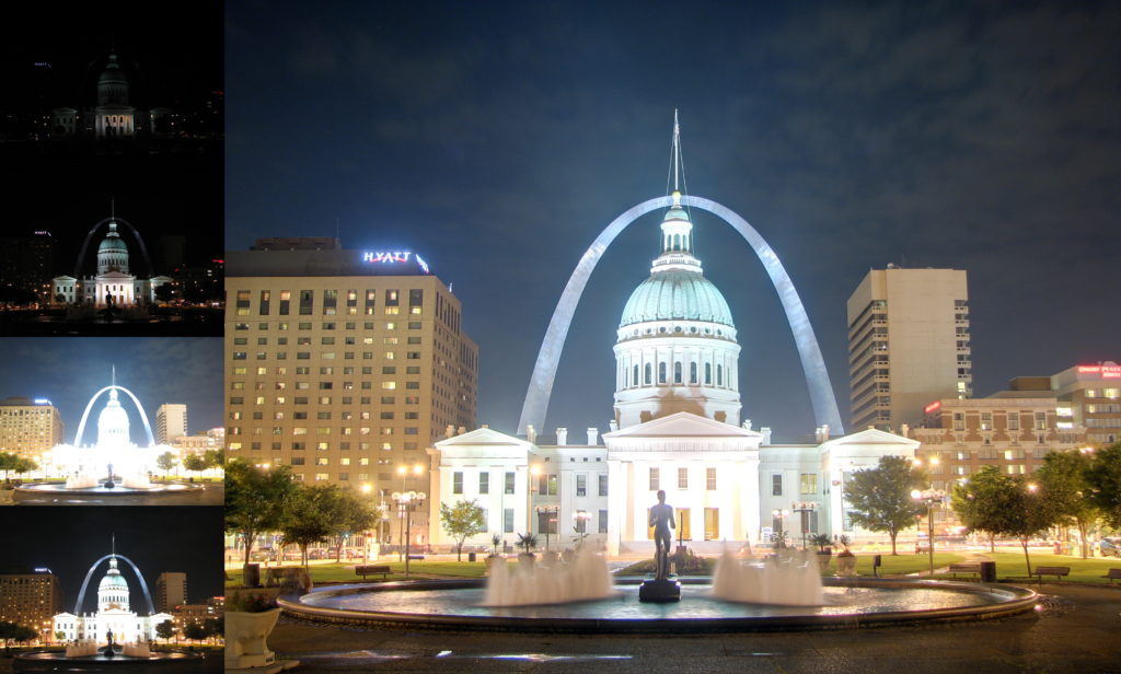
We can also see this effect on the images we used for HDR imaging in our previous post. The four images used to produce the final output are shown on the left and the output image is shown on the right.
Exposure Fusion vs HDR
As you have seen in this post, Exposure Fusion allows us to achieve an effect similar to HDR + Tonemapping without explicitly calculating the HDR image. So we don’t need to know the exposure time for every image and yet we are able to obtain a very reasonable result.
So, why bother with HDR at all? Well, in many cases, the output produced by Exposure Fusion may not be to your liking. There is no knob you can tweak to make it different or better. On the other hand, HDR image captures the original brightness of the scene. If you don’t like a tone mapped HDR image, you try a different tone mapping algorithm.
In summary, Exposure Fusion represents a tradeoff. We are trading off flexibility in favor of speed and less stringent requirements ( e.g. no exposure time is required ).
Image Credits
- The images of Memorial Church are borrowed from Paul Debevek’s HDR page.
- The images of St. Louis Arch is licensed under the Creative Commons Attribution-Share Alike 3.0 Unported license.


