- Introduction
- AI specific features in recent NVIDIA GPUs
2.1 Pascal microarchitecture (2016)
2.2 Volta microarchitecture (2018)
2.3 Turing microarchitecture (Late 2018)
2.4 Ampere microarchitecture (2020)
2.5 Hopper microarchitecture (2022) - CuDNN for framework development
3.1 Who needs cuDNN?
3.2 Convolution in cuDNN - GPU performance for deep learning
- Summary
1. Introduction
Welcome to the second part of this series of blog posts, where we are covering ‘behind the scenes’ of the GPU hardware and CUDA software stack that powers most of deep learning. If you haven’t already, please be sure to read the first part of this series. To quickly recap the learning goals of this two part series, after reading both these posts, you will:
- Learn how a GPU accelerates AI workloads (covered in part 1)
- Understand the features of many generations of NVIDIA GPUs (covered here)
- Choose the right GPU for your training or inference workload (covered here)
- Learn how to write code to maximize GPU utilization (covered here)
In part 1, we introduced the CUDA programming model in detail and implemented a dense layer in CUDA via matrix multiplication. This background will form the basis of the content covered in this post. Having understood the terminology of CUDA, in this post we will dive deep into hardware features for AI acceleration in recent NVIDIA GPUs. In total we will describe the features of five generations of NVIDIA GPUs released over the last 6 years.
A deep understanding of the hardware features will allow you to chose the right GPU for your AI workloads, be it on the cloud or at the edge. After this we will return back to the CUDA software stack, but with a higher level focus on the cuDNN library which enables easy integration of CUDA into machine learning frameworks. Since most deep learning practitioners don’t work directly with either CUDA or cuDNN, we will provide some practical tips to profile and benchmark your AI software directly from the framework itself. Here, we will use PyTorch as an example.
2. AI specific features in recent NVIDIA GPUs
In this section, we will analyze the last 5 generations of NVIDIA GPUs and compare their features for deep learning workloads. We have crystallized all the relevant information from disparate documents and whitepapers into an easily digestible package with the least possible jargon and marketing hype. If you are a senior deep learning engineer or a manager looking to understand which GPU will best serve your needs, this section will be especially helpful to you.
2.1 Pascal microarchitecture (2016)
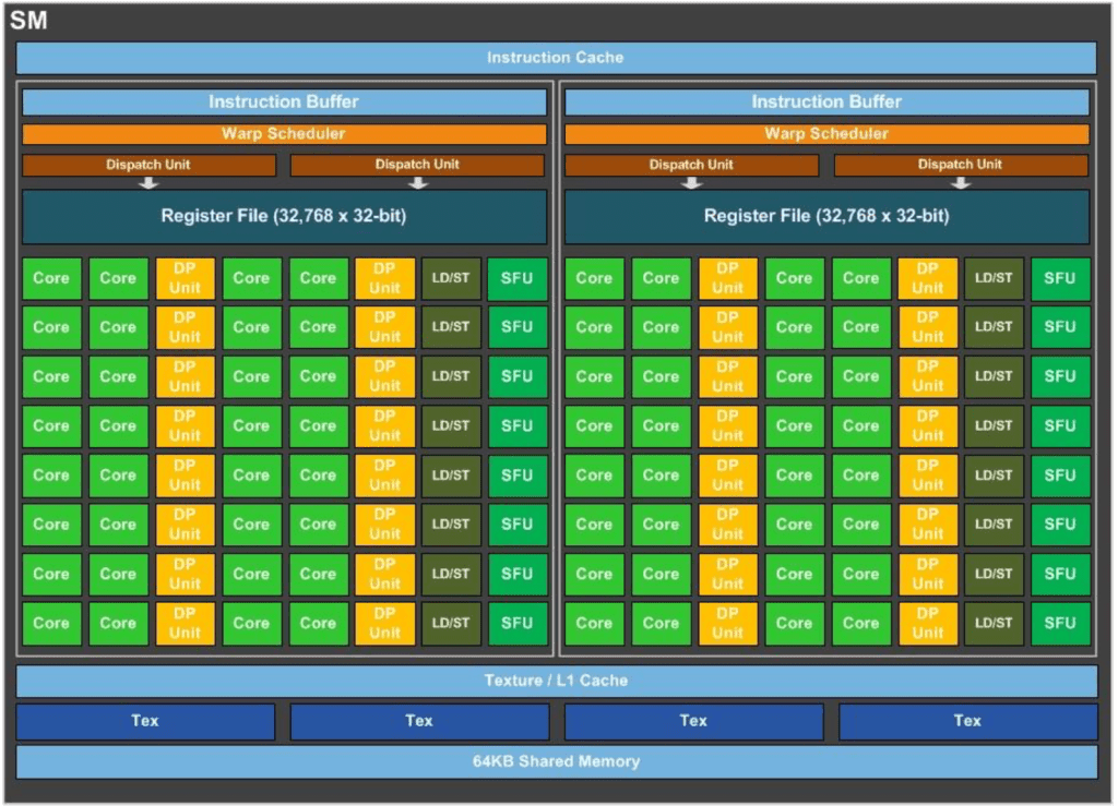
Figure 1. A schematic of the P100 SM
(Source: NVIDIA P100 whitepaper)
We will begin the analysis from the Pascal microarchitecture. Introduced in 2016, the Pascal generation P100 was NVIDIA’s first major datacenter GPU designed for deep learning. The most important feature in Pascal was the introduction of hardware support for float16 calculations. Before Pascal, all GPUs were mainly designed to perform 32-bit or 64-bit floating point calculations, since these were the precisions most important for gaming and high performance computing applications. The P100 design also inspired the well known Jetson TX2.
Figure 1 shows a schematic of the P100 SM. The full P100 GPU contains 56 such SMs.
- The overall P100 SM is composed of two identical processing blocks which shows why NVIDIA calls it a ‘multiprocessor’.
- The green blocks represent CUDA cores,
- Yellow blocks represent CUDA cores dedicated for double precision calculations (almost never used in deep learning, but widely used in HPC workloads such as fluid dynamics simulations).
- SFUs are blocks for special function units which compute functions like sine, cosine, log and exponential. For instance, SFUs will be used for calculating the sigmoid activation.
- ‘Tex’ represents texture memory which was explained in part 1.
- ‘Register file’ represents register memory which is not shared between threads.
- LD/ST represents load/store units which are parts of memory controllers.
- In addition, there are instruction cache, warp scheduler and dispatch units, all of which are not directly controlled by programmers but by firmware within the SMs.
Although both P100 and TX2 continue to be used widely in industry, they are nearing the end of their lives. You should use this generation of hardware if the computational requirements for your application are not expected to increase in the future, or if you are navigating a chip shortage and this is the only hardware you can get your hands on. The Pascal SM forms a great starting point for understanding the next generations.
2.2 Volta microarchitecture (2018)
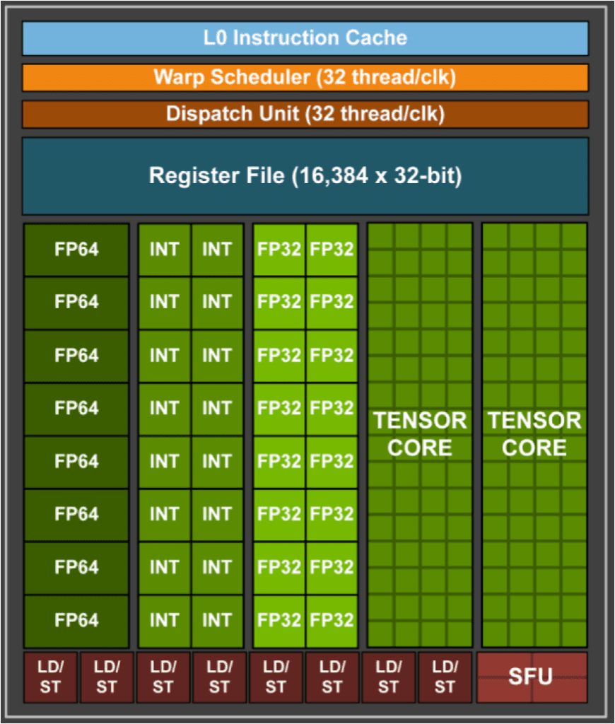
Figure 2. One processing block of the Volta V100 SM, the full SM is composed of four such processing blocks and the full GPU contains 80 SMs (Source: NVIDIA V100 whitepaper)
The Volta microarchitecture was first released at the very end of 2017 and became widely available in 2018. The full SM of the V100 is composed of four processing blocks, one of which is shown in figure 6. The full V100 contains 80 SMs. Armed with the understanding of the P100 SM, several components are readily understandable, such as memory registers, load/store units, CUDA cores and SFUs. The major new innovation in Volta generation was the introduction of Tensor Cores.
A Volta tensor core is a special type of CUDA core designed for Multiply Accumulate (MAC) operations of the form D= A x B + C (where A~D are all 4×4 matrices)

Figure 3. Volta Tensor Core MAC operations (Source: NVIDIA V100 whitepaper)
MAC calculations are used in most deep learning layers since multiplication can be used to implement dense or convolutional layers and addition can be used to apply bias. In Volta TC, A and B must be FP16 matrices but C and D could be either FP16 or FP32. In other words, Tensor Cores accelerate mixed precision operations for deep learning. The secret to this acceleration is that the hardware is designed to perform the two operations of multiplication and addition in one single clock cycle.
These are called Fused Multiply Add (FMA) instructions as illustrated in figure 4. With these enhancements, Volta TCs provide up to 9x enhancement in mixed precision matrix multiplications than Pascal. Volta generation hardware remains a workhorse of several deep learning workloads for various industries and will remain so for at least another couple of years.
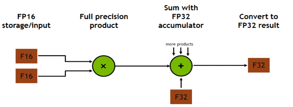
Figure 4. Multiplication and addition happen in one clock cycle also known as FMA.
2.3 Turing microarchitecture (Late 2018)
Turing is a gaming focused GPU architecture very similar to Volta and was released in late 2018. The most important AI specific feature in Turing is that the Turing Tensor Cores support INT8 and INT4 data types, in addition to the FP16 type supported by Volta. This enables INT8 inference on Turing GPUs which is substantially faster than FP16.
Turing GPUs like the RTX20 series are quite popular among AI labs and small teams. In addition, Turing TCs inspired the Jetson AGX Xavier die. In a previous blog post, we showed that INT8 inference on the Jetson Xavier was ~2x faster than fp16 and 10x faster than FP32. These impressive speed ups were enabled by Turing generation tensor cores.
2.4 Ampere microarchitecture (2020)
Introduced in May 2020, the Ampere microarchitecture is the successor to Volta. The A100 GPU is the current flagship CUDA enabled datacenter GPU for deep learning and has 108 SMs. The two major innovations in Ampere for deep learning are:
2.4.1 Third generation Tensor Cores

Figure 5. Performance comparison between Volta and Ampere tensor cores.
(Source: NVIDIA Ampere whitepaper)
The Volta tensor cores were quite limited in the data types they supported. Turing improved on this and with Ampere all the restrictions on the data types supported by tensor cores have been removed. The third generation of tensor cores in Ampere support all data types from binary, INT4, INT8, FP16, TF32 and even FP64. So, with Ampere, deep learning practitioners do not have to use mixed precision training to take advantage of tensor cores. This is great because mixed precision training can sometimes be numerically unstable. With Ampere, full precision TF32 throughput is up to 20x that of Volta.
2.4.2 Structured Sparsity (SS)
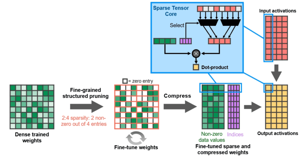
Figure 6. How structured sparsity in Ampere works (Source: Ampere whitepaper)
SS is a principled approach to take advantage of sparsity in neural networks. First, recall that almost all commonly used layers in deep learning can be represented as matrix multiplications. Structured sparsity works on neural networks which have been pruned in a specific way, as explained in figure 6.
- First, train a network as usual (without sparsity) until an acceptable performance is achieved. We now consider one layer of the trained network. Divide the weight matrix of the layer into small patches of 2×2 (quite like we do for max pooling).
- Then for each 2×2 patch of weights, zero out the smallest 2 weights and retain the other 2. This results in a matrix that has exactly half of its elements as zeros.
- There will be some loss in accuracy if we use this pruned weight matrix as is, but with a bit more fine-tuning of the network, the non-zero weights can adjust to compensate for the zeroed out entries.
- The final result of this process is that the fine-tuned weight matrix has almost the same accuracy as the initial dense matrix but requires only half the number of multiplications.
Ampere Structured Sparsity codifies this property of sparse networks into the hardware. During inference, as shown in the blue box of figure 6, the Ampere hardware just skips multiplications wherever zeros are present. Thus, the layer is accelerated by 2x by skipping half of the matrix entries. A couple of things to note here:
- SS can be used with Tensor Cores to achieve a 2x improvement on top of what the 3rd generation tensor cores already offer.
- SS is not enabled in any of the deep learning frameworks, but it is exposed to users via TensorRT 8. Let us know in the comments if you would like to write to us about using SS in practice.
- Although it can also be used during training, SS is usually recommended for inference. You may notice performance drops if you train a model with SS right from the very beginning.
The Ampere microarchitecture was adapted to consumer graphics cards without any major changes, giving gamers access to some pretty hefty AI compute. In particular, even the gaming focused RTX 3090 outperforms the flagship datacenter V100 GPU from a couple of generations ago for most deep learning workflows. If you are short on budget and don’t need all the enterprise features that are only available in datacenter GPUs like V100, the 3090 or 3090Ti may be a good alternative for a small sized team at a research lab or a startup.
The Ampere A100 has inspired the recently released Jetson AGX Orin. Therefore, the Orin’s GPU is much faster than Xavier’s and Orin also supports structured sparsity.
2.5 Hopper microarchitecture (2022)
We covered the features of Hopper in great detail when it was announced in March 2022, but as of writing, the first product H100 is not yet generally available. Let us take a close look at the Hopper SM.
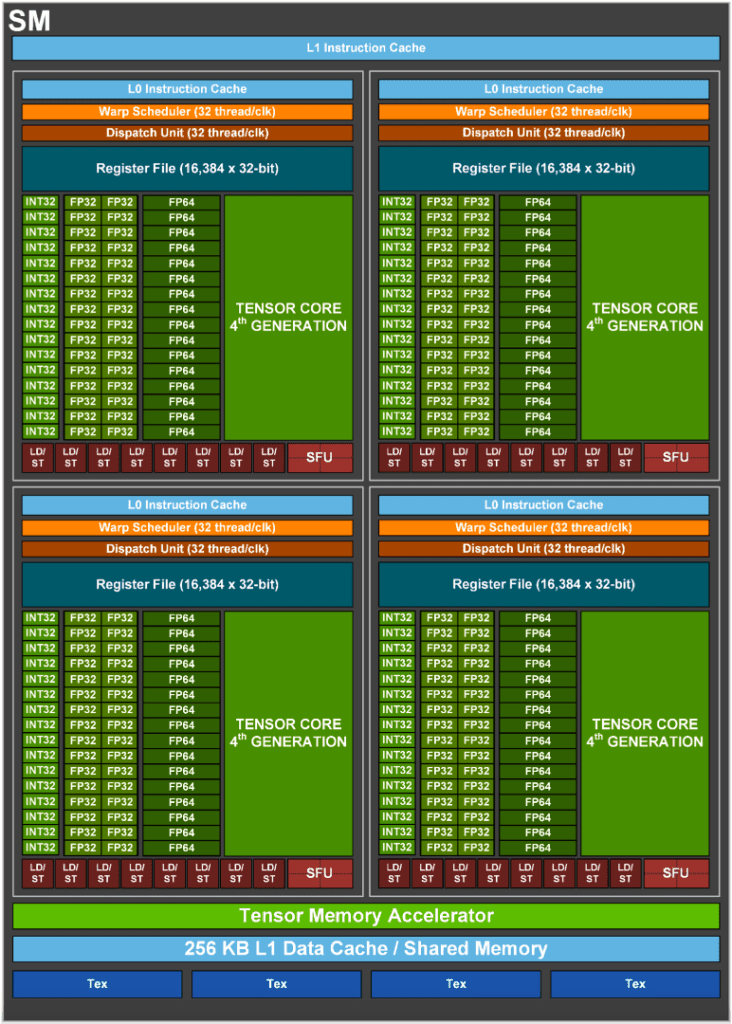
Figure 7. The full Hopper H100 SM, there are a total of 144 SMs
(Source: Hopper whitepaper)
The SM contains the usual suspects, like the floating point compute units, SFUs and memory controllers, but there are a few new features (not all are visible in the above figure):
2.5.1 Support for FP8 data format
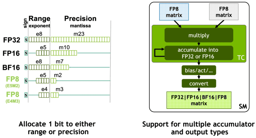
Figure 8. Two variants of 8 bit floating point operations introduced by Hopper.
As shown in figure 12, Hopper introduces two variants of 8 bit floating point precision: 5 exponents with 2 mantissa and 4 exponents with 3 mantissa. These data types are most useful for large language model training, the likes of GPT-3 or PaLM. An advantage of FP8 training is that during inference, there is no need to convert the model to a lower precision and the model trained can be used as is, guaranteeing absolutely no loss in performance.
2.5.2 Fourth generation tensor cores
The Hopper tensor cores offer double the performance of Ampere tensor cores at the same clock frequency. Since the H100 supports FP8, has more SMs and a higher boost frequency, the overall matrix multiply throughput from H100 is 6x that of A100 (FP8 on Hopper v/s FP16 on Ampere).
2.5.3 Tensor Memory Accelerators (TMA)
As we noted in part 1, memory access takes much longer than computation. Memory access can become a bottleneck for large models with billions of parameters. TMAs sit between the global memory and shared memory in the CUDA programming model hierarchy. They accelerate memory transfers by asynchronously transferring data to shared memory while the CUDA threads do some other work. This allows data to be available to every thread without having to wait for a transfer to be completed. Since Hopper isn’t quite available yet, it is unclear if TMA acceleration will be built into frameworks like PyTorch and TensorFlow.
2.5.4 DPX instructions for dynamic programming
Dynamic programming is an important class of computational workload most commonly used in genomics and robotics. The DPX instructions accelerate these problems by 7x over A100. NVIDIA notes that this would be useful, for example, in accelerating the calculation of optimal paths for robots in a warehouse.
2.5.5 Thread Block Clusters
We discussed earlier that all threads in a block run only on one SM and can share memory among themselves. As GPUs scale to over a hundred SMs, more fine grained control over resources is required to execute massive computing workloads. To this end, Hopper introduces a new extension of the CUDA programming model, called Thread Block Clusters (TBCs). In figure 1 of part 1, we saw the CUDA thread hierarchy goes from Thread → Block → Grid.
TBCs sit between blocks and grid, so the new hierarchy is Thread → Block → Thread Block Cluster → Grid. The advantage of having TBCs is that clusters can contain blocks running on different SMs. Hopper also contains additional mechanisms to let blocks from one cluster share memory among themselves without going through the global memory. This is called Distributed Shared Memory. We can see that such features can accelerate attention layers for large transformer models when calculating softmax, for example, since the softmax of a vector element depends not only on it’s own value but also the sum of exponentials of all the values in the vector.
2.5.6 Transformer Engine (TE)
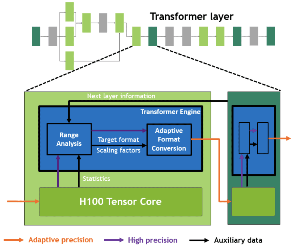
Figure 9. Hopper transformer engine (Source: Hopper whitepaper)
This is perhaps the most important feature of the Hopper architecture. We are covering it at the end because all the previous background is necessary to understand transformer engines. TEs neatly integrate all the above new features introduced in Hopper to accelerate transformer training.
During forward pass of an attention layer, activations from the previous layer are used to calculate attention scores using tensor cores at a mix of FP16 and FP8 precisions. If FP8 is used carelessly, it could result in loss of accuracy. Particularly, FP16 → FP8 conversion can lead to a large loss in precision as we have fewer bits to represent a given value. To minimize this loss in precision, a software module (in the firmware of the SM) analyzes the range of activations produced by this layer and the next layer (black arrows) and uses this information to scale the conversion from FP16 → FP8. Conceptually, this is similar to INT8 calibration performed for inference.
The range analysis and format conversion allow most computation and data transfers to be performed in FP8 and only the metadata about minimum, maximum etc. are kept in FP16. Therefore, every layer is accelerated optimally according to the range of activations it produces.
Hopper is at the bleeding edge of AI hardware as of the time of writing. Even most of NVIDIA’s SDKs (such as TensorRT) have not yet been updated to take advantage of all of Ampere’s features. This will change over this year and the next.
You should not consider Hopper for your deployments for now unless you absolutely need the highest possible performance and do not have any budgetary constraints. However, if you are reading this article long after it is published, please verify how many of the features explained above are supported in frameworks and whether your specific workload or application benefits from them.
3. CuDNN for framework development
Have you ever wondered why NVIDIA has never developed their own framework like PyTorch for TensorFlow despite having the resources to do it? Couldn’t they optimize performance on their GPUs better than PyTorch or TensorFlow developer teams?
This curious situation is explained by a library called cuDNN. We have reviewed the fundamental CUDA concepts that underlie every GPU computation. However, the full CUDA library is too complex and low-level for most programmers to use directly. Knowing this, as early as 2014, NVIDIA released cuDNN, a C++ library built on top of CUDA which provides highly optimised routines for frequently used operations in deep learning.
With cuDNN, a programmer doesn’t have to deal directly with CUDA cores, SMs, warps, etc. Rather, they can just treat cuDNN functions as regular C++ functions and call them as they would with any other library.
cuDNN provides framework developers with an easy way to add GPU support for their framework without knowing the details of CUDA and GPU hardware. Thus, by creating a ‘framework for frameworks’, NVIDIA ensured that their GPUs were supported by all major AI/ML frameworks and libraries.
3.1 Who needs cuDNN?
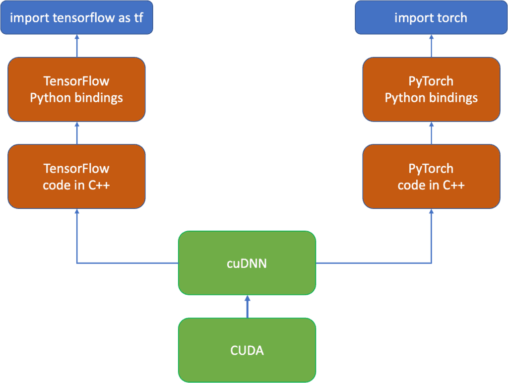
Figure 10. Deep learning framework software stack
The most common use case for cuDNN is for framework development such as TensorFlow or PyTorch. As a framework developer you will work with cuDNN and almost never directly with CUDA. The only case for direct CUDA usage is if you are trying to implement a custom layer or if you want to merge a few layers for computational efficiency. Therefore, if you are not planning to develop your own framework, you do not need to know cuDNN. However, if you are comfortable with C++, learning cuDNN is easy and will definitely boost your confidence.
3.2 Convolution in cuDNN
Just like CUDA, cuDNN is quite vast. Here, we will take the example of a convolutional layer and review how PyTorch uses cuDNN to implement it. CuDNN uses the cudnnConvolutionForward function to expose convolution operation. This function has the following signature in cuDNN:
cudnnStatus_t cudnnConvolutionForward(
    cudnnHandle_t                       handle,
    const void                         *alpha,
    const cudnnTensorDescriptor_t       xDesc,
    const void                         *x,
    const cudnnFilterDescriptor_t       wDesc,
    const void                         *w,
    const cudnnConvolutionDescriptor_t  convDesc,
    cudnnConvolutionFwdAlgo_t           algo,
    void                               *workSpace,
    size_t                              workSpaceSizeInBytes,
    const void                         *beta,
    const cudnnTensorDescriptor_t       yDesc,
    void                               *y)
Although we have not introduced all the concepts behind cuDNN, most of the inputs to this function are quite understandable. For example, cudnnTensorDescriptor_t is some kind of a struct describing properties of the input tensor, cudnnFilterDescriptor_t describes filter properties, and cudnnConvolutionDescriptor_t specifies some properties of the convolution operation. One important parameter is cudnnConvolutionFwdAlgo_t. This is the low level implementation by which the convolution calculations should be performed. The following implementations of convolution are available:
- GEMM: This method implements convolution as a matrix to matrix multiplication
- Implicit GEMM: This is similar as above, except that the matrices being multiplied are never explicitly created in memory. This saves memory.
- Implicit precomp GEMM: Similar to above, except that in this implementation, some commonly required values are pre-calculated. This requires a bit of extra memory but can save computational time.
- Direct: This method implements convolution with a sliding window approach and is slower than GEMM based methods.
- FFT: This method takes advantage of the mathematical relation between convolution and the Fast Fourier Transform to implement convolution
- FFT tiling, and
- Winograd: this method pre-computes some statistics of the convolution kernel and uses them to accelerate the convolution operation.
Let us look at how PyTorch uses cuDNN to implement convolution on the GPU. This link contains the exact location in PyTorch code where the forward implementation of convolution is described in a file named `cuda_op_convolution.cu`. A few lines of the code are reproduced below:
CUDNN_ENFORCE(cudnnConvolutionForward(
        state->cudnn_handle(),
        cudnnTypeWrapper<T_X>::kOne(),
        bottom_desc_,
        X.template data<T_X>(),
        filter_desc_,
        filter.template data<T_W>(),
        conv_desc_,
        algo_,
        state->workspace().get(cudnn_ws_nbytes_),
        cudnn_ws_nbytes_,
        cudnnTypeWrapper<T_Y>::kZero(),
        top_desc_,
        Y->template mutable_data<T_Y>()));
The code just calls cudnnConvolutionForward and passes references to input tensor and convolution filters. As a short exercise, take a look at the equivalent definition of convolution operation in TensorFlow and try to understand how the forward and backward passes of the convolutional layer are implemented. OpenCV’s DNN module also uses cuDNN under the hood with the convolution operation defined here. In contrast to TensorFlow and PyTorch, OpenCV DNN does not define backward pass for convolution since OpenCV’s DNN module supports only inference and not training.
A major advantage of cuDNN is that whenever new hardware such as tensor cores are added to GPUs, NVIDIA updates cuDNN to take advantage of that hardware under the hood, and the framework developers don’t need to modify anything. As a result, end-users of PyTorch automatically get enhanced performance when using newer versions of CUDA (cuDNN is bundled within CUDA, so you usually do not need to install it separately). This is equally true for TensorFlow.
Although cuDNN is quite a low-level library from the point of view of ML engineers, it is convenient and high-level for framework engineers, as it gives them lots of flexibility and performance. As a deep learning engineer, you do not have to worry about all the intricacies of the above code walkthrough but we recommend taking a look at the cuDNN documentation.
4. GPU performance for deep learning
CUDA has an extensive suite of debugging and profiling tools like cuda-memcheck, cuda-gdb, nvprof, nsys, ncu to name a few. Since deep learning practitioners do not work with CUDA and cuDNN directly, the developers of frameworks have integrated profiling tools within the frameworks so that users can understand how well their code is optimized. Here we will take a look at PyTorch profiling tools.
4.1 How to profile your code for DL training.
You can profile your code with a few simple steps and visualize the results with Tensorboard. First, install the tensorboard PyTorch profiler with
pip install torch_tb_profiler
The next step is to slightly modify a typical PyTorch training loop to profile the resource usage statistics. This is done by creating a `profile` object to log both CPU and CUDA events and export the logs into a format that can be read by tensorboard. This allows the profiler to record both the CPU and GPU parts of the execution and identify bottlenecks in training.
from profiler_demo_utils import *
#importing * is not good practice, but simplifies
#this demo. Please do not imitate this :-)

class VisionTrainer(object):
	def __init__(self, net, dm):
		pass
		self.net=net
		self.dm=dm
		self.writer=SummaryWriter()
		self.criterion=nn.CrossEntropyLoss()
		self.optimizer=optim.AdamW(self.net.parameters(), lr=1e-6)
		self.savepath=None

	def train(self, epochs, save, profiler=None):
		pass
		eval_interval=200 #evaluate every 200 steps
		self.savepath=save
		device = torch.device('cuda') if torch.cuda.is_available() else torch.device('cpu')
		train_loader, valid_loader = self.dm.train_loader, self.dm.valid_loader #ignore test loader if any

		self.net.to(device).train()

		if has_apex:
			self.net, self.optimizer = amp.initialize(self.net, self.optimizer,
										opt_level='O2', enabled=True)

		step=0

		get_accuracy=lambda p,y: (torch.argmax(p, dim=1) == y).to(torch.float).mean().item()

		for epoch in range(epochs):
			estart=time.time()
			for x,y in train_loader:
				with record_function("training_events"): #record these as training_events
					self.optimizer.zero_grad()

					x=x.to(device)
					y=y.to(device)

					pred = self.net(x)

					loss = self.criterion(pred,y)

					#print(loss.item())
					self.writer.add_scalar('Training Loss', loss.item(), step)

					with amp.scale_loss(loss, self.optimizer) as scaled_loss:
						scaled_loss.backward()

					#loss.backward()

					torch.nn.utils.clip_grad_norm_(self.net.parameters(), 0.01)
					self.optimizer.step()
					acc=get_accuracy(pred, y)
					step+=1
					self.writer.add_scalar('Training Accuracy', acc, step)

				if step%eval_interval==0:
					with record_function("evaluation_events"): #record these as evaluation_events
						self.net.eval()
						valoss=[]
						vaacc=[]
						with torch.no_grad():
							pass
							for imgs, ys in valid_loader:
								imgs=imgs.to(device)
								ys=ys.to(device)
								preds=self.net(imgs)
								vacc=get_accuracy(preds, ys)
								vloss=self.criterion(preds, ys)
								#pdb.set_trace()
								valoss.append(vloss.flatten().item())
								vaacc.append(vacc)

						self.writer.add_scalar('Validation Loss', np.mean(valoss), step)
						self.writer.add_scalar('Validation Accuracy', np.mean(vaacc), step)
						self.net.train()

				if profiler:
					profiler.step()

			self.save(epoch)
			eend=time.time()
			print('Time taken for last epoch = {:.3f}'.format(eend-estart))

	def save(self, epoch):
		if self.savepath:
			path=self.savepath.format(epoch)
			torch.save(self.net.state_dict(), path)
			print(f'Saved model to {path}')


def main():
	dm=CIFAR10_Manager('./cf10')

	#Just change name to one of the following:
	#resnet18, resnet50, mobilenetv3, densenet, squeezenet, inception
	mname='resnet50'
	net=VisionClassifier(nclasses=10, mname=mname)

	trainer=VisionTrainer(net,dm)

	with profile(activities=[ProfilerActivity.CPU, ProfilerActivity.CUDA],
		record_shapes=True,
		schedule=schedule(
        wait=1,
        warmup=1,
        active=2),
        on_trace_ready=torch.profiler.tensorboard_trace_handler('./runs'),
		profile_memory=True,
		use_cuda=True) as prof:

		trainer.train(epochs=1, save='models/cf10_{}.pth', profiler=prof)

if __name__=='__main__':
	main()
We are now ready to profile and visualize the results. Just run the training script and open a tensorboard window in your browser.

Figure 11. Screenshot of PyTorch profiler for ResNet-50 fine-tuning on CIFAR-10.
The profiler gives a very detailed view of the operations performed in the training loop. The blue box in figure 11 contains many perspectives you may choose to look at. However, the profiler provides the most important statistics in the overview section (see red box). For example in this case the profiler shows that only 30% of the CUDA kernels run on tensor cores. Moreover, GPU utilization is just ~18%. The green box shows a recommendation to improve performance in easy to understand terms. In this case, the profiler advises us to increase the batch size to better use the GPU.
5. Summary
In this blog post, we built upon the foundation laid in part 1 of this series and reviewed the most relevant features for deep learning in recent NVIDIA GPUs.
Starting from the Pascal generation introduced in 2016, we traced the evolution of GPU hardware and understood exactly how certain features such as tensor cores, structured sparsity and transformer engines work. This knowledge is far and beyond what a typical engineer would need in their daily job, but it is helpful to know all these details if you are planning to invest in high-end GPUs for your team or just want to rent GPU instances on the cloud.
After understanding the details of the hardware features of GPUs, we learnt about cuDNN, which was developed by NVIDIA to simplify CUDA integration into deep learning frameworks. cuDNN is used by framework developers, and we discussed specific examples showing implementations of the convolutional layer in PyTorch, TensorFlow and OpenCV’s DNN module.
Finally, we discussed some practical tips for using profiler tools directly from frameworks using python to understand the performance of your code. We saw the specific case of the PyTorch profiler.
It is perfectly possible to build a successful career in deep learning without knowing anything we have described in this short two-part series of blog posts. However, sooner or later, you will realize that to advance your career and stand apart from other engineers, you need to either (a) keep up to date with the latest research papers and algorithms or (b) develop a much deeper understanding of the tools of your trade so you can solve problems that others cannot.
This series is a small step to help you in the latter direction. We hope you have enjoyed reading the post and learnt something. Please let us know in the comments or on any social media platform which topics mentioned here would you want to read more about in the future.



100K+ Learners
Join Free OpenCV Bootcamp3 Hours of Learning