TensorFlow Model Optimization Toolkit – A Deep Dive

In the previous posts of the TFLite series, we introduced TFLite and the process of creating a model. In this post, we will take a deeper dive into the TensorFlow Model Optimization. We will explore the different model optimization techniques supported by the TensorFlow Model Optimization Toolkit (TF MOT). A detailed performance comparison of the optimized models has also been provided.

This is the third post in the TensorFlow Lite series with the following.

1. TensorFlow Lite: Model Optimization for On-Device Machine Learning
2. TensorFlow Lite Model Maker: Create Models for On-Device Machine Learning
3. TensorFlow Model Optimization Toolkit: Deeper Dive into Model Optimization

1. TensorFlow Model Optimization Toolkit
2. Fine-tuning Base Model
3. Code Explanation
   1. Import Libraries
   2. Load Dataset
   3. Resize Dataset
   4. Import Keras Model
   5. Train the Model
   6. Pruning
   7. Weight Clustering
   8. Quantization Aware Training
4. Comparison of the Optimized Models
   1. Test Accuracy
   2. Model Size

1. TensorFlow Model Optimization Toolkit

The TensorFlow Model Optimization Toolkit is a suite of tools for optimizing ML models for deployment and execution. Among many uses, the toolkit supports techniques used to:

• Reduce latency and inference costs for cloud and edge devices (e.g. mobile, IoT).
• Deploy models to edge devices with restrictions on processing, memory, power consumption, network usage, and model storage space.
• Enable execution and optimization for existing hardware or new special-purpose accelerators.

2. Fine-tuning Base Model

All of the optimization techniques we will discuss will require training of the model. To benchmark the performance of the optimized model, we will fine-tune the base model we trained in our earlier TensorFlow Lite: Model Optimization article.

Click here to download the source code to this post

3. Code Explanation

Let’s start by installing the TensorFlow Model optimization Toolkit with the following commands. We are using Google Collab, so the rest of the packages are already available. Please use requirements.txt file from the downloaded code for setting up a local environment.

# For google colab.!pip install -q tensorflow-model-optimization

# For a local environment.
!pip install -r requirements.txt 

3.1 Import Libraries

# Importing necessary libraries and packages.
import os
import numpy as np
import tensorflow as tf
from tensorflow import keras
import tensorflow_datasets as tfds
from tensorflow.keras.models import Model
import tensorflow_model_optimization as tfmot
from tensorflow.keras.layers import Dropout, Dense, BatchNormalization
%load_ext tensorboard

3.2 Load Dataset

The dataset can be directly loaded from TensorFlow Dataset (tfds). We are importing the Cat vs Dog dataset. The dataset is split into Training, Validation and Testing sets with a split ratio of 0.7:0.2:0.1. The as_supervised parameter is kept True since we need the labels of the images for classification. 

# Loading the cat vs dog dataset.
(train_ds, val_ds, test_ds), info = tfds.load('cats_vs_dogs', split=['train[:70%]', 'train[70%:90%]', 'train[90%:]'], shuffle_files=True, as_supervised=True, with_info=True)

Let us now have a look at the dataset information provided in tfds.info(). The dataset has two classes labeled as ‘cat’ and ‘dog’ with 16283, 4653, 2326 training, validation and testing images.

# Printing dataset information.
print("Number of  Classes: " + str(info.features['label'].num_classes))
print("Classes : " + str(info.features['label'].names))
NUM_TRAIN_IMAGES = tf.data.experimental.cardinality(train_ds).numpy()
print("Training Images: " + str(NUM_TRAIN_IMAGES))
NUM_VAL_IMAGES = tf.data.experimental.cardinality(val_ds).numpy()
print("Validation Images: " + str(NUM_VAL_IMAGES))
NUM_TEST_IMAGES = tf.data.experimental.cardinality(test_ds).numpy()
print("Testing Images: " + str(NUM_TEST_IMAGES))

3.3 Resize dataset

We are taking 16 as batch size and 224×224 as image size so that the dataset can be processed effectively and efficiently.

# Defining batch size and input image size.
batch_size = 16
img_size = [224, 224]

# Resizing images in the dataset.
train_ds = train_ds.map(lambda x, y: (tf.image.resize(x, img_size), y))
val_ds = val_ds.map(lambda x, y: (tf.image.resize(x, img_size), y))
test_ds = test_ds.map(lambda x, y: (tf.image.resize(x, img_size), y))

Let’s make sure to use buffered prefetching to yield data from the disk. Prefetching overlaps the preprocessing and model execution of a training step. Doing so reduces the step time to the training and the time it takes to extract the data.

train_ds = train_ds.cache().batch(batch_size).prefetch(buffer_size=10)
val_ds = val_ds.cache().batch(batch_size).prefetch(buffer_size=10)
test_ds = test_ds.cache().batch(batch_size).prefetch(buffer_size=10)

3.4 Import Keras Model

We will import the Keras model and then compile it to see the final model’s summary. We have used Adam Optimizer with an initial learning rate of 0.0001, sparse categorical cross-entropy as loss function and accuracy as the metric.

# Importing the keras model.
model = tf.keras.models.load_model('/content/drive/MyDrive/TFLiteBlog/models/model.h5')
# Compiling the model.
model.compile( optimizer=tf.keras.optimizers.Adam(0.0001), loss =tf.keras.losses.SparseCategoricalCrossentropy(from_logits=False), metrics = ["accuracy"])model.summary()

Output:

====================================================================
Total params: 4,740,453
Trainable params: 4,697,406
Non-trainable params: 43,047
____________________________________________________________________

We will be using Model Saving Callback and the Reduce LR Callback, similar to the TensorFlow Lite Model on device machine learning.

1. Model Saving Callback saves the model with best validation accuracy.
2. Reduce LR Callback reduces the learning rate by a factor of 0.1 if validation loss remains the same for 3 consecutive epochs.

# Defining file path.
filepath = '/content/model.h5'

# Defining Model Save Callback and Reduce Learning Rate Callback for achieving better results.
model_save = tf.keras.callbacks.ModelCheckpoint(
    filepath,
    monitor="val_accuracy",
    verbose=0,
    save_best_only=True,
    save_weights_only=False,
    mode="max",
    save_freq="epoch")

reduce_lr = tf.keras.callbacks.ReduceLROnPlateau(monitor='loss', factor=0.1, patience=3, verbose=1, min_delta = 5*1e-3,min_lr = 5*1e-9,)

callback = [model_save, reduce_lr]

3.5 Train the Model

Now we will train the model using the model.fit() method. We will pass the training dataset and validation dataset and train the model for 2 epochs.

# Training the model for 2 epochs.
model.fit(train_ds, epochs=2, steps_per_epoch = (len(train_ds)//batch_size), validation_data=val_ds, validation_steps = (len(val_ds)//batch_size), shuffle = False, callbacks=callback)

Let’s check the model’s performance on the test set.

# Evaluating the model on the test dataset.
_, baseline_model_accuracy = model.evaluate(test_ds, verbose=0)
print(Baseline Keras Model Test Accuracy:', baseline_model_accuracy*100)

Output:

Baseline Keras Model Test Accuracy : 98.49 %

3.6 Pruning

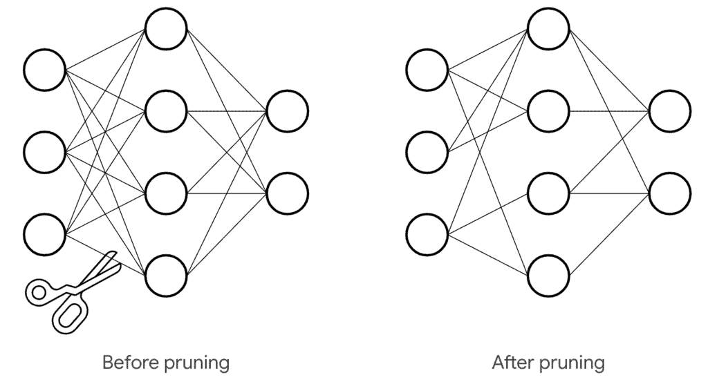
Pruning of a model involves the removal of parameters within the models that have minimal impact on its predictions. In weight pruning, unnecessary values in the weight tensors are eliminated. The neural network parameters’ values are set to zero to remove the unnecessary connections between the layers of a neural network. This is done during the training process to allow the neural network to adapt to the changes. Effective pruning can reduce the model size significantly. It doesn’t affect runtime latency.

Here, we will only prune the final dense layers. We will clone the base model and apply pruning to its final dense layers.

# Dense layers train with pruning.
def apply_pruning_to_dense(layer):
  if isinstance(layer, tf.keras.layers.Dense):
    return tfmot.sparsity.keras.prune_low_magnitude(layer)
  return layer
# Using `tf.keras.models.clone_model` to apply `apply_pruning_to_dense`  to the layers of the model.
model_for_pruning = tf.keras.models.clone_model(model, clone_function = apply_pruning_to_dense)

Let’s see the Model Summary. 

# Printing model summary.model_for_pruning.summary()

Output:

=====================================================================
Total params: 5,428,715
Trainable params: 4,697,406
Non-trainable params: 731,309

We can observe that the model parameters have increased here. This is because tfmot adds non-trainable masks for each of the weights in the network to denote if a given weight should be pruned. The masks are either 0 or 1.

Let’s now compile the model having the same loss function and metrics as that of the base model.

# Compiling model for pruning.
model_for_pruning.compile(
      optimizer=tf.keras.optimizers.Adam(0.0001),
      loss =tf.keras.losses.SparseCategoricalCrossentropy(from_logits=False),                     metrics = ["accuracy"])

Here, tfmot.sparsity.keras.UpdatePruningStep is required during training as it updates pruning wrappers with the optimizer step, and tfmot.sparsity.keras. PruningSummaries provides logs for tracking progress and debugging.

# Defining the Callbacks and assigning the log directory.
logdir = 'content/logs'
callbacks = [
  tfmot.sparsity.keras.UpdatePruningStep(),
  tfmot.sparsity.keras.PruningSummaries(log_dir=logdir),
]

We will now fine-tune this model on the training dataset for two epochs.

# Fine tuning the model.
model_for_pruning.fit(train_ds, batch_size=batch_size, epochs=2, validation_data=val_ds, callbacks=callbacks)

Let’s evaluate this pruned model.

# Evaluating pruned Keras model on the test dataset._, model_for_pruning_accuracy = model_for_pruning.evaluate(test_ds, verbose=0)
print('Baseline Keras Model Test Accuracy:', baseline_model_accuracy*100)
print('Pruned Keras Model Test Accuracy:', model_for_pruning_accuracy*100)

Output:

Baseline Keras Model Test Accuracy: 98.49 %
Pruned Keras Model Test Accuracy: 99.14 %

The logs show the progression of sparsity on a per-layer basis.

# Tensorboard logs.
%tensorboard --logdir={logdir}

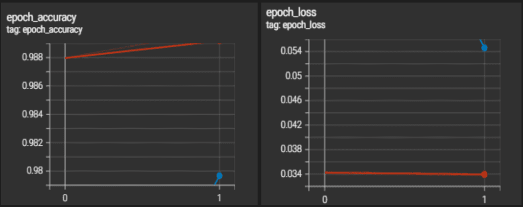
The model is exported and saved in Keras’s .h5 format. The strip_pruning() is necessary since it removes every tf.Variable that pruning only needs during training, which would otherwise add to model size during inference. Further, pruning makes most of the weights zeros, which is added redundancy that standard compression algorithms can utilize to compress the model further.

# Exporting pruned Keras modelmodel_for_export = tfmot.sparsity.keras.strip_pruning(model_for_pruning)
tf.keras.models.save_model(model_for_export, '/content/pruned_keras_model.h5', include_optimizer=False)

Let us now print the model summary of the exported model. Here we can see that exported pruned Keras model parameters are the same as the baseline models. This is because the size of the weight metrics returned is the same as the base model, but most of the weights are zero.

Output:

pruned_keras_model.summary()
=====================================================================
Total params: 4,740,453
Trainable params: 4,697,406
Non-trainable params: 43,047
_____________________________________________________________________

3.7 Weight Clustering

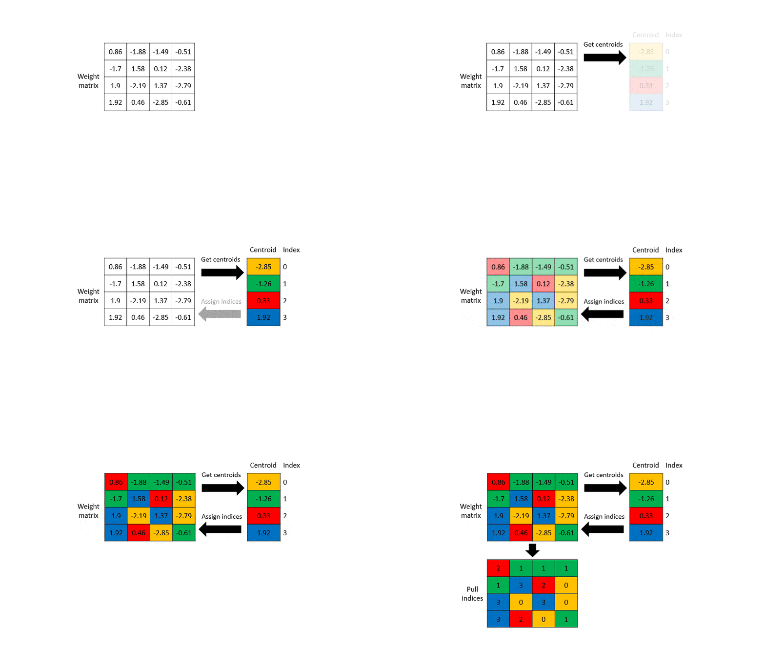
Clustering works by grouping the weights of each layer in a model into a predefined number of clusters, then sharing the centroid values for the weights belonging to each individual cluster. This reduces the number of unique weight values in a model, thus reducing its complexity. As a result, clustered models can be compressed more effectively, providing deployment benefits similar to pruning. To cluster a model, it needs to be fully trained first before passing it to the clustering API. As we have already trained our baseline model, we can now proceed to cluster our model.

Let’s define clustered weights and Centroid Initialization using TFMOT.

# Defining clustered weights using TFMOT.
cluster_weights = tfmot.clustering.keras.cluster_weights
CentroidInitialization =tfmot.clustering.keras.CentroidInitialization

The number_of_clusters parameter is the number of cluster centroids to be formed when clustering a layer/model. Here we have set number_of_clusters to  16. This will ensure that each weight tensor has no more than 16 unique values.  The cluster_centroids_init parameter determines how the cluster centroids will be initialized. 

• In RANDOM initialization centroids are sampled using the uniform distribution between the minimum and maximum weight values in a given layer. 
• In DENSITY_BASED initialization density-based sampling takes place. 
• In the LINEAR initialization cluster, centroids are evenly spaced between the minimum and maximum values of a given weight.

# Setting clustering parameters.clustering_params = { 'number_of_clusters': 16,  'cluster_centroids_init': CentroidInitialization.LINEAR}

# Cluster a whole model.
clustered_model = cluster_weights(model, **clustering_params)

Let’s compile the weight-clustered model.

# Compiling clustered model.
clustered_model.compile(optimizer=tf.keras.optimizers.Adam(0.0001), loss =tf.keras.losses.SparseCategoricalCrossentropy(from_logits=False), metrics = ["accuracy"])

Print the clustered model summary.

Output:

=====================================================================
Total params: 9,203,973
Trainable params: 4,698,494
Non-trainable params: 4,505,479

Here also, we can notice model parameters almost getting doubled. The reason is similar to the case of pruning. For fine-tuning the clustered model, TF MOT adds masks to the weights, doubling the number of parameters.

Now we will fine-tune the weight-clustered model. We will finetune the model for 2 epochs.

# Fine-tune model.
clustered_model.fit(train_ds, batch_size= batch_size, epochs=2, validation_data = val_ds)

Let’s evaluate the clustered model on the test set.

# Evaluating the Fine-tuned clustered model._, clustered_model_accuracy = clustered_model.evaluate(test_ds, verbose=0)
print('Baseline Keras Model Test Accuracy:', baseline_model_accuracy*100)
print('Pruned Keras Model Test Accuracy:', model_for_pruning_accuracy*100)print('Clustered Keras Model Test Accuracy:', clustered_model_accuracy*100)

Output:

Baseline Keras Model Test Accuracy: 97.76 %
Pruned Keras Model Test Accuracy: 99.35 %
Clustered Keras Model Test Accuracy: 70.16 %

Export the clustered model and save it in Keras’s .h5 format.  Here we will make use of the strip_clustering()  that removes the masks that were added during the training and returns the weight metrics of a similar size as that of the base model.

# Saving the clustered model.
final_model = tfmot.clustering.keras.strip_clustering(clustered_model)
clustered_keras_file = '/content/weight_clustered_keras_model.h5'
tf.keras.models.save_model(final_model, clustered_keras_file, include_optimizer=False)

Let’s now print the model summary for the saved clustered model to check the number of parameters in the model. Here we can see that the clustered model parameters are the same as that of the based model after strip clustering.

# Printing clustered model summary.
clustered_model.summary()
=====================================================================
Total params: 4,740,453
Trainable params: 4,697,406
Non-trainable params: 43,047
_____________________________________________________________________

3.8 Quantization-Aware Training

As we move to a lower precision from float, we generally notice a significant accuracy drop as this is a lossy process. This loss can be minimized with the help of quant-aware training. Quant-aware training simulates low precision behavior in the forward pass, while the backward pass remains the same. This induces some quantization error which is accumulated in the total loss of the model, and hence the optimizer tries to reduce it by adjusting the parameters accordingly. This makes our parameters more robust to quantization, making our process almost lossless.

Here also we will quantize only the final dense layers.

# Only the dense layers are quantized.
def apply_quantization_to_dense(layer):
  if isinstance(layer, tf.keras.layers.Dense):
    return tfmot.quantization.keras.quantize_annotate_layer(layer)
  return layer

# Cloning base model and applying quantization on dense layers.
annotated_model = tf.keras.models.clone_model(
    model,
    clone_function=apply_quantization_to_dense,
)

quant_aware_model = tfmot.quantization.keras.quantize_apply(annotated_model)
quant_aware_model.summary()

Output:

=====================================================================
Total params: 4,740,470
Trainable params: 4,697,406
Non-trainable params: 43,064

Here the number of non-trainable parameters has increased. This is because TF MOT adds some masks to layers to specify whether they should be quantized or not.  Let’s compile the model.

# Compiling the quant aware model.quant_aware_model.compile(
      optimizer=tf.keras.optimizers.Adam(0.0001), loss =tf.keras.losses.SparseCategoricalCrossentropy(from_logits=False), metrics = ["accuracy"]
)

We will now fine-tune the model.

# Fine-tuning quantization aware trained model.
quant_aware_model.fit(train_ds, batch_size=batch_size, epochs=2, validation_data=val_ds)

Let’s evaluate this freshly trained model on the test set.

# Evaluating quantization aware trained model on test dataset.
_, quant_aware_model_accuracy = quant_aware_model.evaluate(test_ds, verbose=0)
print('Baseline Keras Model Test Accuracy:', baseline_model_accuracy*100)
print('Pruned Keras Model Test Accuracy:', model_for_pruning_accuracy*100)
print('Clustered Keras Model Test Accuracy:', clustered_model_accuracy*100)
print('Quantization Aware Trained Model Test accuracy:', quant_aware_model_accuracy*100)

Output:

Baseline Keras Model Test Accuracy: 98.49%
Pruned Keras Model Test Accuracy: 99.14%
Clustered Keras Model Test Accuracy: 70.16%
Quantization Aware Trained Model Test accuracy: 99.35%

Let’s save this model in Keras format. 

# Saving quantization aware trained Keras model.
quant_aware_model.save('/content/quant_aware_keras_model.h5')

Further, to load the Quantization Aware trained Keras Model, it needs to be deserialized. quantize_scope() deserializes the Keras model to load. Let’s now load the Quantization Aware trained Keras Model and view its model summary.

Output:

quant_aware_model.summary()
=====================================================================
Total params: 4,740,470
Trainable params: 4,697,406
Non-trainable params: 43,064
_____________________________________________________________________

We can see that after deserializing the Keras Model the number of parameters is the same as that of the baseline model. 

4. Comparison of the Optimized Models

4.1 Test Accuracy

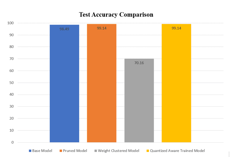
The pruned model and the quantized aware-trained model have similar test accuracy, and their performance on the test set is better than the base model. The test accuracy of the weight-clustered model is significantly lower than that of the base model.

4.2 Model Size

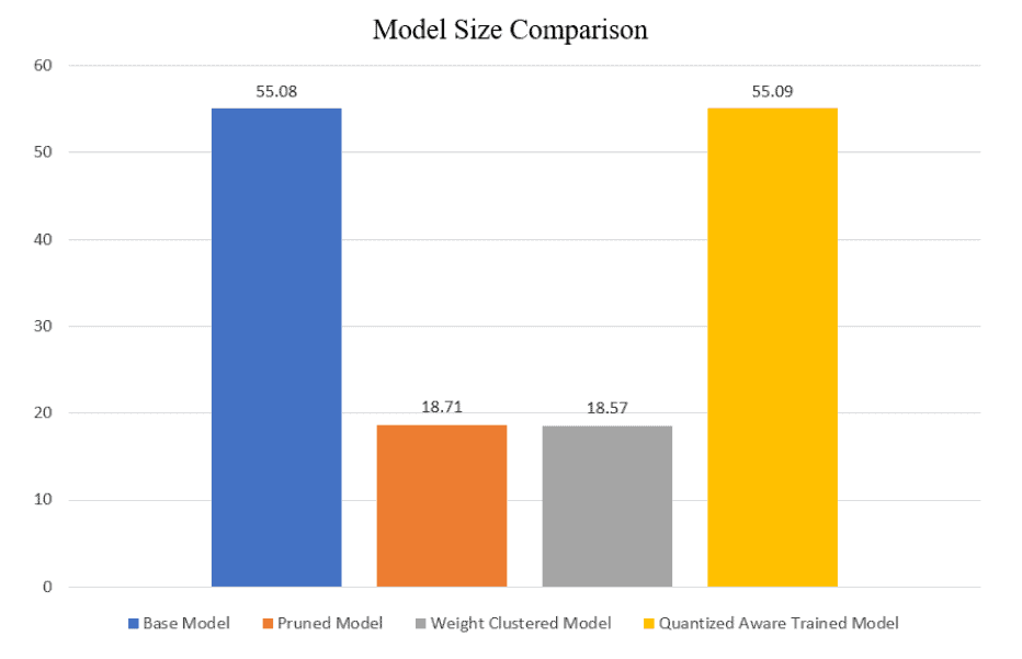
As we can see up to 3x of size reduction was observed in the pruned and weight-clustered model. The quantized aware model has a size similar to that of the base model.