This article is the first part of the Mastering LLMs series, Here we will discuss what LLMs are, their use cases, and the tasks they perform. We will also explain the underlying Transformer architecture and the intuition behind it. Then, we will cover different fine-tuning techniques, such as full fine-tuning and parameter-efficient fine-tuning. We will also introduce you to the concept of Quantization which will help you save some computational resources.

What is Generative AI?
Generative AI is a type of artificial intelligence technology that can produce various types of content, including text, imagery, audio, and synthetic data. The simplicity of new user interfaces has been driving the recent popularity of generative AI, enabling users to create high-quality texts, images, and videos in seconds.
Generative AI is a subset of Machine learning in which models have learned statistical patterns underlying vast amounts of data generated by humans. For example, researchers have trained Large Language Models on trillions of words over many weeks or months, using large amounts of computing power to understand natural language.
Use Cases of LLMs
Large Language Models (LLMs), typically referred to as “Large Language Models,” are advanced artificial intelligence models designed to understand and generate human-like text. They undergo training on vast amounts of text data to learn the structure and patterns of human language. LLMs have a wide range of applications beyond chat tasks. While chatbots have gained significant attention, LLMs excel in next-word prediction, which forms the foundation for various capabilities. Some common use cases of LLMs include:
- Summarizing text.
- Translating texts (for example, converting text to code).
- Generating essays based on given topics.
- Extracting specific information from text.
In addition to these applications, augmenting LLMs is an active area of research focusing on connecting LLMs with external data sources and invoking external APIs. This integration allows the model to leverage information that it may not have learned during its pretraining, further enhancing its capabilities. We’ll discuss such techniques in the upcoming blogs.
LLMs offer a powerful tool for natural language generation and have the potential to revolutionize various domains by automating tasks that require language understanding and generation.
Demystifying Transformers: A Deep Dive
Why Transformers?
You might wonder, how do LLMs learn so well? What is the most crucial ingredient for a LLM? The answer is the Transformer architecture introduced in the paper “Attention is All You Need”. Of course, there are other elements as well which are also equally important such as massive data that LLMs use and the training algorithms used to train the LLMs, but the Transformer architecture is the key component that allows modern LLMs to leverage the other components so well.
Using transformers leads to a dramatic increase in performance over previously used RNNs for generative AI tasks. The key to such enhanced performance of transformers lies in their ability to learn the relevance and context of all the words in a sentence.
This learning process occurs through weighted connections between each word and every other word within a given sentence. During training, the model learns the weights of these connections, known as attention weights. This capability is commonly referred to as self-attention.
From Words to Vectors
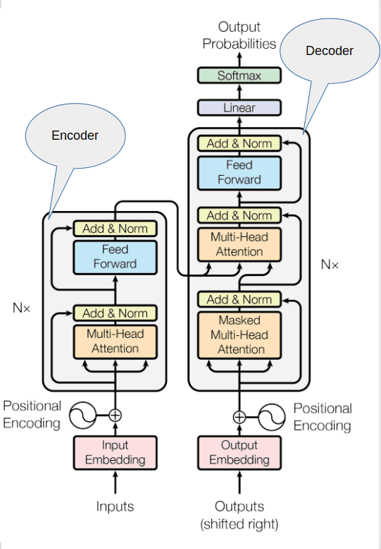
As you can see the architecture mainly consists of an encoder and a decoder. Machine learning models are big statistical calculators and work with numbers. So, the first step before passing texts is to tokenize the input sequences. The process of tokenization maps each word to a number from a dictionary of words, some tokenizers map the words in the English dictionary to numbers while some map parts of words. The key is that once a tokenizer is chosen for training, you must use the same tokenizer for your text generation task.
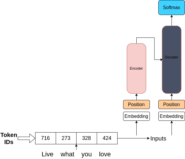
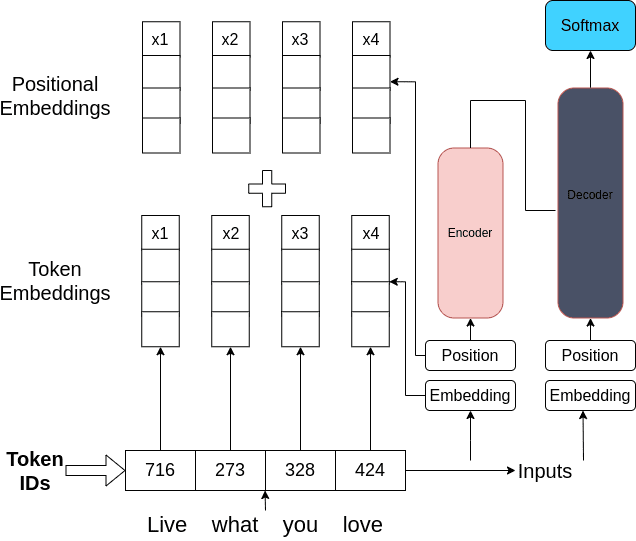
The second step is to pass these tokens to the embedding layer, this is a trainable layer where each token in the vocabulary is assigned a high-dimensional vector that learns to encode the meaning and context of individual tokens in the input sequence. By encoding the words into high-dimensional vectors the model mathematically tries to understand language.

The next step is to encode the position of each word in the input sequence. After this step, the vectors from the embedding layer and position encoding layer are summed up and passed to the self-attention layer.
Self-Attention: Understanding Relationships Within Text
The self-attention layer, as seen earlier, learns the relationship between one word and all the other words in the input sequence. This is achieved by assigning attention weights to all the connections present between parts of the input sequence.
Both the encoder and the decoder consist of multiple self-attention heads, by this I mean that there are multiple layers, each of which learns the attention weights between different words of the input sequence independently. The intuition here is that each head will probably learn a different aspect of language. For example, one head might focus on the sentiment involved in a sentence while the other head might focus on the relationship between named entities in a sentence. Each of these weights is learned during training by the model. Initially, the weights are assigned randomly, given sufficient data and time these weights learn different aspects of language.
After passing through the multi-headed self-attention layer, attention weights are applied to the input sequence. Subsequently, the sequence undergoes processing by a feed-forward network layer, which generates a vector of logits containing probabilities for each word in the vocabulary. This vector can be passed into the softmax layer to get probability scores for each word, with various methods available to select the final output. To understand the underlying mathematical formulations of the attention mechanism you can check out Understanding Attention Mechanism in Transformer Neural Networks.
Putting It All Together: An Overview of the Transformer
Now that we understand the components, let’s look at the end-to-end prediction process. Consider a translation task, each word in the input sequence is tokenized and processed through the encoder’s multi-headed self-attention layers. The output from the encoder influences the decoder’s self-attention mechanisms. A start-of-sequence token is added to trigger the prediction of the next token. The process continues until a stopping condition is met, resulting in a sequence of tokens that can be detokenized to form the output word sequence.
To summarize the architecture on a high level, the encoder encodes inputs(prompts) into a deep understanding of the structure and meaning of the input and produces one vector per input token and the decoder accepts input tokens and generates new tokens using the understanding provided by the encoder.
Fine Tuning Techniques
Instruction Fine Tuning
In contrast to pre-training where you train the LLM on vast amounts of unstructured textual data via self-supervised learning, fine-tuning is a supervised learning process where you update the weights using a dataset with labeled examples. This helps you in improving the model’s performance on specific tasks. The labeled examples could be examples of a sentiment analysis task, a translation task, a summarization task, or some other task, it could also be a combination of the above tasks. The labeled examples contain two parts:
- Prompt (for sentiment analysis task, it could be: I am feeling good today.)
- Completion (for the above prompt it would be: Positive.)
Many publicly available datasets can be used for training language models however most of them are not formatted as instructions. Luckily, several prompt template libraries provide templates for various tasks for various datasets. These libraries can process popular datasets for creating data that can be used for instruction fine-tuning.
Instruction fine-tuning where all the model weights are updated is known as full fine-tuning. Fine-tuning like this requires you to store all the model weights and therefore this requires the same amount of computing power as required during pre-training. You can explore this method in full detail and get your hands dirty by building some interesting applications at Fine Tuning T5: Text2Text Transfer Transformer for Building a Stack Overflow Tag Generator and Text Summarization using T5: Fine-Tuning and Building Gradio App
Multi-task Fine Tuning
In multi-task fine-tuning, we essentially fine-tune the model on multiple tasks simultaneously. This requires large amounts of examples for training. Tasks suitable for multi-task fine-tuning include Sentiment Analysis, Text Summarization, Question Answering, Machine Translation, etc.
Multi-task fine-tuning allows models to learn and generalize across a spectrum of challenges, ultimately improving their overall performance.
Parameter Efficient Fine-Tuning (PEFT)
What is PEFT?
LLMs can be quite large, with the largest ones requiring hundreds of gigabytes of storage. And to be able to perform full finetuning on an LLM, you not only need to store all the model weights, but also gradients, optimizer states, forward activations, and temporary states throughout the training process. This can require a substantial amount of computing power, which can be quite challenging to obtain.
Instead of updating every single weight during training like full-finetuning, parameter-efficient methods focus on a small subset. This can be done by:
- Fine-tuning specific layers or components: Only relevant parts are adjusted rather than retraining the entire model.
- Freezing LLM weights and adding new components: The original model becomes read-only, while additional layers or parameters are introduced and trained specifically for the task.
Overall, only about 15-20% of the original parameters are updated, allowing parameter-efficient fine-tuning to be done even on a single GPU with less computational resources.
Since most of the LLM weights are only slightly modified or left unchanged, the risk of catastrophic forgetting is reduced significantly.
Classes of PEFT
The 3 main classes of PEFT methods are as follows:
- Selective methods: These methods specialize in fine-tuning just a portion of the initial LLM parameters. You have various options to decide which parameters to modify. You can opt to train specific components of the model, specific layers, or even specific types of parameters.
- Reparameterization methods: These methods reduce the number of parameters to train by creating new low-rank transformations of the original network weights. One commonly used technique of this type is LoRA, which we will explore in the next part of the Mastering LLM series.
- Additive methods: These methods perform fine-tuning by keeping the original LLM weights unchanged and incorporating new trainable components. There are two primary approaches in this context. Adapter methods introduce new trainable layers into the model’s architecture, usually within the encoder or decoder components, following the attention or feed-forward layers. Conversely, soft prompt methods maintain the fixed and frozen model architecture while focusing on manipulating the input to enhance performance. This can be achieved by adding trainable parameters to the prompt embeddings or by keeping the input unchanged and retraining the embedding weights.
Evaluation Methods
In traditional machine learning methods, we can assess the model’s performance on a training set or validation set because the output is deterministic. We can use metrics such as accuracy, precision, recall, f1-score, etc to determine how well the model is performing. However, in the case of LLMs, this can be difficult because the output is non-deterministic, and language-based evaluation can be quite challenging.
For example, consider the following sentences, “The weather is beautiful today” and “The weather is wonderful today”. Both of the above sentences have similar meanings, but how do we measure this similarity? for example, consider the following sentence, “The weather is horrible today”, now this sentence has an opposite meaning compared to the other two. But all three sentences had just one-word differences. We humans can easily distinguish between these sentences but we need a structured, well-defined method to measure the similarity between different sentences to train LLMs. ROUGE and BLEU, are two widely used evaluation metrics for different tasks.
ROUGE ((Recall-Oriented Understudy for Gisting Evaluation) Score
It is commonly used for text summarization tasks. It is used to objectively evaluate the similarity between machine-generated summaries and the reference summary provided by humans for a longer text. Let’s see some types of ROUGE scores.
- ROUGE-1 Score: It measures the overlap of single words in machine-generated text and reference text. It calculates quantities like precision, recall, and F1 score based on the number of overlapping words. While this method can measure how similar two texts are it might be a little deceiving. For example, consider the following reference sentence “It’s cold in here” and then, consider the following two machine-generated sentences, “It’s very cold in here” and “It’s not cold in here”, the measured value for both of these sentences will be the same, however, one of them has opposite meaning compared to the reference text.
- ROUGE-N Score: It measures the overlap of n-grams (n consecutive words from a given sentence) in machine-generated text and reference text. It calculates quantities like precision, recall, and F1-score based on the number of overlapping n-grams. Since this metric takes bi-grams and n-grams for calculations, intuitively one can see that it takes the position of words into account as well.
- ROUGE-L Score: This is another common ROUGE score where we use the length of the longest common subsequence irrespective of the order for calculating quantities such as precision, recall, and F1-score which are collectively known as ROUGE scores.
BLEU (Bilingual Evaluation Understudy) Score
It is a metric for automatically evaluating machine-translated text. The BLEU score is a number between zero and one that measures the similarity of the machine-translated text to a set of reference translations. In simple terms, you can say that it is a geometric mean of precision values over a range of n-gram sizes.
Some Qualitative Insights
Now, let’s quantitatively see how these metrics change for different pairs of texts. Consider the following reference text, machine-generated texts, and the corresponding metrics:
| Reference Text | Artificial intelligence is transforming various industries, including healthcare and finance. |
| Prediction 1 | AI is revolutionizing different sectors, like healthcare and finance. |
| Prediction 2 | Artificial intelligence is transforming industries such as healthcare and finance. |
| Prediction 3 | Artificial intelligence is transforming various industries, including healthcare and finance. |
| Prediction | BLEU Score | ROUGE-1 Score | ROUGE-2 Score | ROUGE-L Score |
|---|---|---|---|---|
| Prediction 1 | 0.23708 | 0.42105 | 0.23529 | 0.42105 |
| Prediction 2 | 0.44127 | 0.8 | 0.5555 | 0.8 |
| Prediction 3 | 1.0 | 1.0 | 1.0 | 1.0 |
You can see how the BLEU score and the ROUGE scores improve as we get closer and closer to the reference text. You can download the code below, play around with the reference texts and predicted texts, and see how these metrics change for yourself.
Quantization
Why Quantization?
LLMs have millions or billions of parameters and each of these parameters is represented with a certain number of bits usually 32 bits or 16 bits. For example, let’s consider a model with 1 billion parameters with all of its parameters stored with 32-bit floating point numbers. Each parameter in this model will take up 4 bytes of memory. So, in total, 1 Billion parameters will take up 4 ∗ 109 bytes of memory, equivalent to 4GB of memory.
This means that to store a 32-bit model with 1 Billion parameters, you’ll need 4GB of memory. If you want to train such a model then you’ll require additional memory for storing the gradients, activations, optimizer states, and other temporary variables needed by your functions. This can easily lead to around 20 extra bytes of memory per model parameter. After accounting for all these additional memory requirements during training, you’ll need approximately 6 times the amount of GPU RAM for training such a model (approx. 24GB), on top of this, you will need some memory for your data. This is too much for edge devices.
The Quantization Trade-Off
Then, What options do you have to reduce the memory required for training? One technique that you can use to reduce the memory is called Quantization. By replacing 32-bit floating point numbers with 16-bit or even 8-bit integers, quantization significantly reduces the memory demands of large language models and neural networks.
To ensure accuracy and flexibility, model weights, activations, and parameters are typically stored in the 32-bit floating-point format by default. Quantization projects the original 32-bit floating point numbers into a lower precision space using scaling factors. However, the downside to this technique is that you lose out on the performance by decreasing the precision of the original parameters. The more you decrease the precision the more you lose out on the performance.
Popular Quantization Techniques
Now, let’s try to understand how you store a number in a 32-bit floating point representation and also look at how you can quantize them to a 16-bit floating point representation. Among various data types, floating point numbers are predominantly employed in deep learning due to their ability to represent a wide range of values with high precision. Typically, a floating point number uses n bits to store a numerical value. These n bits are further partitioned into three distinct components:
- Sign: This bit indicates the positive or negative nature of the number. It uses one bit where 0 indicates a positive number and 1 signals a negative number.
- Exponent: The exponent is a segment of bits that represents the power to which the base (usually 2 in binary representation) is raised. The exponent can also be positive or negative, allowing the number to represent very large or very small values.
- Significant/Mantissa: The remaining bits are used to store the significand, also referred to as the mantissa. This represents the significant digits of the number. The precision of the number heavily depends on the length of the significand.
This design allows floating point numbers to cover a wide range of values with varying levels of precision. The formula used for this representation is:
(−1)sign∗ baseexponent∗ mantissa
To understand this better, let’s look into some of the most commonly used data types in deep learning and see how you transform a float32 number to a float16 and bfloat16 number:
- FP32 uses 32 bits to represent a number: 1 bit for the sign, 8 for the exponent, and the remaining 23 for the significand. While it provides a high degree of precision, the downside of FP32 is its high computational and memory footprint. Consider the following FP32 representation of 2.71828:

(−1)0 ∗ 2128−127 ∗ 1.35914003 = 2.71828007
- FP16 uses 16 bits to store a number: 1 is used for the sign, 5 for the exponent, and 10 for the significand. Although this makes it more memory-efficient and accelerates computations, the reduced range and precision can introduce numerical instability, potentially impacting model accuracy. Look at the quantized FP16 representation of 2.71828:

(−1)0 ∗ 2128−127 ∗ 1.358398 = 2.716796
- BF16 is also a 16-bit format but with 1 bit for the sign, 8 for the exponent, and 7 for the significand. BF16 expands the representable range compared to FP16, thus decreasing underflow and overflow risks. Despite a reduction in precision due to fewer significant bits, BF16 typically does not significantly impact model performance and is a useful compromise for deep learning tasks. Look at the quantized float 16 representation of 2.71828:

(−1)0 ∗ 2128−127 ∗ 1.3515625 = 2.703125
Conclusion
In this article, we covered the Transformer architecture and built an intuition on how the Transformer architecture understands natural language. Then we explored several fine-tuning techniques such as full-finetuning and parameter-efficient fine tuning (PEFT). We saw that there are several PEFT techniques that you can use to finetune an LLM on your unique data with as little as a single GPU. We also covered the concept of quantization which allows us to reduce the model’s memory footprint and accelerates the inference process. At the end of this article, we discussed some important evaluation metrics that act as guides for LLMs to learn a given task systematically.
References
- Attention is All You Need
- BLEU: a Method for Automatic Evaluation of Machine Translation
- ROUGE: A Package for Automatic Evaluation of Summaries
- Scaling Down to Scale Up: A Guide to Parameter-Efficient Fine-Tuning






100K+ Learners
Join Free OpenCV Bootcamp3 Hours of Learning