Supervised Learning has been dominant for years, but its reliance on labeled data—a costly and time-consuming resource—creates challenges, especially in areas like medical imaging. On the other hand, Unsupervised Learning, even though it doesn’t use labeled data still lacks a clear structure and hence struggles to achieve meaningful patterns. Contrastive Learning strikes a balance here. It learns from unlabeled data, yet creates its structure by focusing on similarities and differences. Instead of needing explicit categories, it groups similar items, enabling models to understand complex patterns
Modern approaches often blend self-supervised and supervised elements by refining learned representations with human-labeled data, creating a semi-supervised framework. In this way, it combines the scalability of unsupervised learning with the precision of supervised learning. This allows researchers to pre-train on large unlabeled datasets and fine-tune on smaller labeled ones, combining the scalability of unsupervised learning with the precision of supervised methods. As a result, Contrastive Learning has become a powerful tool for overcoming the limitations of traditional learning paradigms.
As this article is solely based on the global concept of contrastive Learning, let’s have a very brief idea about what Contrastive Learning is. We will also explain every non-general technical term used in this article.
- Contrastive Learning
- Some of the Popular Technologies Using Contrastive Learning
- The Roots of Contrastive Learning: A Journey Through Time
- Limitations and Ongoing Research in Contrastive Learning
- Key Milestones in the Evolution of Contrastive Learning Frameworks
- SimCLR (Simple Framework for Contrastive Learning of Visual representations)
- Student-Teacher model aka Knowledge Distillation
- BYOL (Bootstrap Your Own Latent)
- Key differences between SimCLR and BYOL
- BYOL Implementation code
- Key Takeaways
- Conclusion
- References
Contrastive Learning
Contrastive Learning is a self-supervised technique that empowers models to learn representations from unlabeled data. Instead of relying on labels, it focuses on pretraining by aligning an encoder to extract meaningful features. These learned embeddings are later used for downstream tasks like classification, object detection, or segmentation, where labels are available.
The key idea is simple:
- Bring positive pairs closer: Semantically similar items (e.g., two views of the same object) should be close in the embedding space.
- Push negative pairs apart: Semantically dissimilar items (e.g., views of different objects) should be far apart.
Let’s take a look at an example:
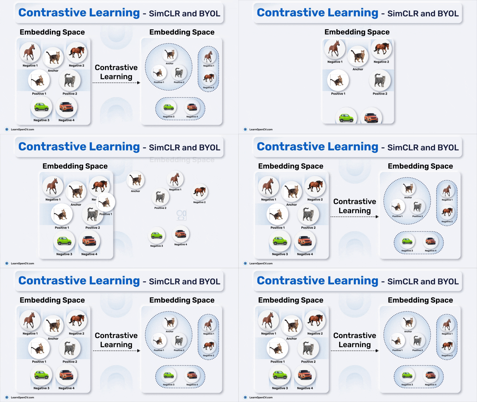
Anchor: the input image (photo of a cat)
Positive Pair: Semantically similar image as the original image (augmented view of the same cat or another different photo from the same class to which the cat belongs)
Negative Pair: Semantically dissimilar image (photo of a car or horse)
The model learns to pull the positive pair closer to the anchor while pushing the negative farther away, creating a well-structured embedding space that clusters similar items and separates dissimilar ones. This approach makes Contrastive Learning a foundational tool for pretraining in machine learning, paving the way for tasks where labeled data is scarce but representations are crucial.
Positive pairs are often generated by applying augmentations (e.g., cropping, rotating) to the same data point while Negative pairs will be the representations of all other data points available in the batch or dataset except for the representations already there in the positive pair we’re considering.
A contrastive loss function (e.g., Contrastive Loss, Triplet Loss, NT-Xent Loss) ensures that embeddings for positive pairs are closer together, while embeddings for negative pairs are pushed farther apart. Contrastive Loss explicitly calculates the distance between positive and negative pairs and penalizes them based on their similarity. Triplet Loss extends this by considering an anchor, a positive, and a negative, optimizing to minimize the anchor-positive distance and maximize the anchor-negative distance. The NT-Xent Loss (Normalized Temperature-Scaled Cross-Entropy Loss), used in SimCLR, scales cosine similarity scores to a meaningful range using temperature, effectively optimizing the alignment and separation of embeddings.
Some of the Popular Technologies Using Contrastive Learning
- SimCLR, MoCo, BYOL, etc. (Computer Vision).
- CLIP and ALIGN (Cross-Modal Learning).
- Sentence-BERT (NLP).
- Spotify and Pinterest (session-based recommendation systems).
- Tesla Autopilot (scene understanding and object detection)
- Wav2Vec (Speech Processing).
The Roots of Contrastive Learning: A Journey Through Time
Early Foundations: Contrastive Divergence Algorithm (2002)
The origins of Contrastive Learning trace back to 2002, with Geoffrey Hinton’s Contrastive Divergence (CD) algorithm. It gave the idea of comparing the data in a way that reduces the difference between the real data distribution and the model’s learned distribution.
Word2Vec and Early Embeddings (2013)
Though not explicitly called Contrastive Learning, Word2Vec inspired modern techniques by:
- Introduction of negative sampling to distinguish between positive and negative pairs.
- Generalizing dense embeddings – evolved from word representations to images, videos, and more.
- Leveraging unlabeled data, similar to modern self-supervised methods.
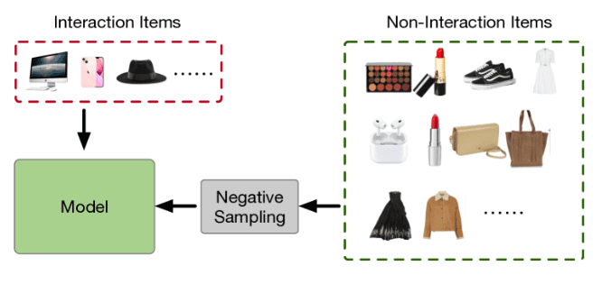
Modern Contrastive Learning (2018-2020)
The technique gained prominence with methods like:
- SimCLR (2020): Published by researchers at Google Brain, this framework defined modern contrastive learning for unsupervised representation learning on images.
- MoCo (2019): Momentum Contrast by Facebook AI.
These methods solidified the term “Contrastive Learning” in its current context, focusing on learning representations by contrasting positive and negative pairs. Contrastive Learning as a specific technique for representation learning was popularized between 2018 and 2020 with models like SimCLR and MoCo.
Contrastive Learning’s first prominent use in the Computer Vision domain was shown in the paper “Unsupervised Feature Learning via Non-Parametric Instance Discrimination” by Wu et al. in Facebook AI Research (FAIR) which defined the task of Instance Discrimination, where each image was treated as its class, and augmentations of the same image were contrasted with other images. This is the precursor to modern frameworks like SimCLR and MoCo.
Next, we’ll explore the limitations of modern Contrastive Learning. While some have been addressed, others remain open research topics. Then, we’ll dive into SimCLR, the framework that popularized modern Contrastive Learning, followed by an introduction to BYOL, a more advanced and optimized approach, including its implementation code.
Modern Contrastive Learning, despite its impressive capabilities and developments, still faces some limitations. Many of these have been addressed with partial solutions or are active research areas. Below is a detailed explanation of the limitations and how researchers address them.
Limitations and Ongoing Research in Contrastive Learning
Contrastive Learning has revolutionized self-supervised representation learning, but like any other approach, it comes with challenges. These limitations have spurred innovations and ongoing research aimed at improving its effectiveness and scalability.
Dependence on Negative Samples
Contrastive learning relies on negative samples, which are computationally expensive and prone to errors from False Negatives. Innovations like BYOL and Barlow Twins eliminate the need for negatives by focusing on positive pairs or feature decorrelation.
High Computational and Memory Costs
Methods like SimCLR need large batch sizes which eventually makes it resource-heavy. MoCo addresses this with a memory queue, while distillation techniques enable lightweight models for easier deployment.
Lack of Semantic Understanding
Instance-level discrimination (treating each data point as a unique distinct class) limits contrastive learning’s grasp of semantic relationships. Techniques like Prototypical Contrastive Learning (PCL) and Contrastive Clustering group similar instances, improving semantic understanding.
Scalability to Multimodal Data
Aligning multimodal data like text, audio, and images is complex. Frameworks like CLIP and ALIGN align embeddings across modalities, pushing the boundaries of multimodal contrastive learning.
Over-sensitivity to Hard Negatives
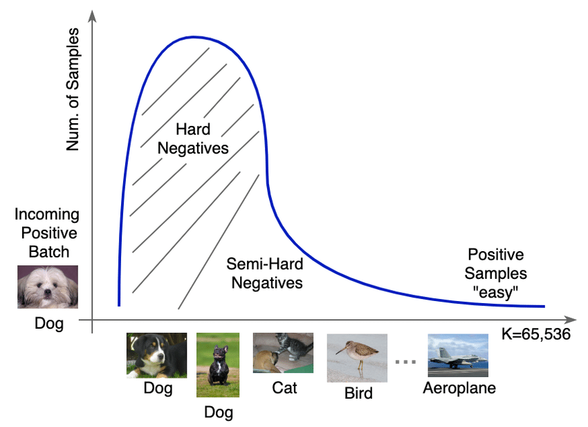
Hard negatives (pairs that are visually or semantically similar to positives) can destabilize training while enriching it. For example, distinguishing between similar-looking dog breeds might confuse the model. Adaptive mining and loss functions strategically manage hard negatives, balancing stability with detailed learning.
Sensitivity to Dataset Bias
Bias in datasets skews representations, causing overfitting. Debiased contrastive learning uses hard-negative mining (helps the model learn to focus on more hard-negative samples) to ensure diversity and data balancing ensures diverse and unbiased learning.
| Limitations | Solutions and Ongoing Research | Trying to achieve |
| Dependence on Negative Samples | BYOL, Barlow Twins | Simplified training process |
| Computational Requirements | MoCo, Distillation | Reduced memory usage |
| Lack of Semantic Understanding | Hybrid Approaches, PCL | Better task-specific performance |
| Multimodal Scalability | CLIP, ALIGN | Extension to multi-modal tasks |
| Sensitivity to Hard Negatives | Curriculum Learning, Adaptive Loss Functions | Better training dynamics |
| Dataset Bias | Debiased Learning, Balanced Datasets | Reduced Bias |
Key Milestones in the Evolution of Contrastive Learning Frameworks
Before discussing SimCLR, we need to know a little bit more about the technologies and evolutions that led to the development of SimCLR.
Earlier to MoCo (Momentum Contrast) and SimCLR, several other foundational frameworks laid the groundwork for Contrastive Learning, but these frameworks were not as scalable or efficient. Let’s explore the evolution of contrastive learning frameworks and the key developments leading up to MoCo.
| Year | Framework | Key Contribution |
| 2018 | Non-Parametric Instance-level Discrimination | The first framework to treat each image as a unique class using contrastive learning. Introduced the memory bank |
| 2018 | Contrastive Predictive Coding (CPC) | Used the contrastive loss to predict future latent states in sequences |
| 2019 | PIRL | Learned pretext-invariant representations using contrastive learning |
| 2020 | MoCo | Solved the stale memory bank problem with a momentum encoder and a dynamic queue |
Just one month after the release of MoCo, SimCLR was introduced.
SimCLR (Simple Framework for Contrastive Learning of Visual representations)
SimCLR is based on contrastive self-supervised learning algorithms without requiring any specialized architectures or memory bank and aims to maximize agreement between augmented views of the same image (positive pairs) while minimizing agreement with views of other images (negative pairs).
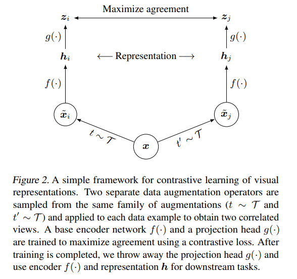
SimCLR Training Workflow
A detailed explanation of the SimCLR’s training workflow can be found in the next section (SimCLR’s Algorithm) of this article.
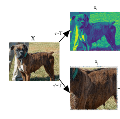
- Augment input images into x1 and x2 (refer to the image below).
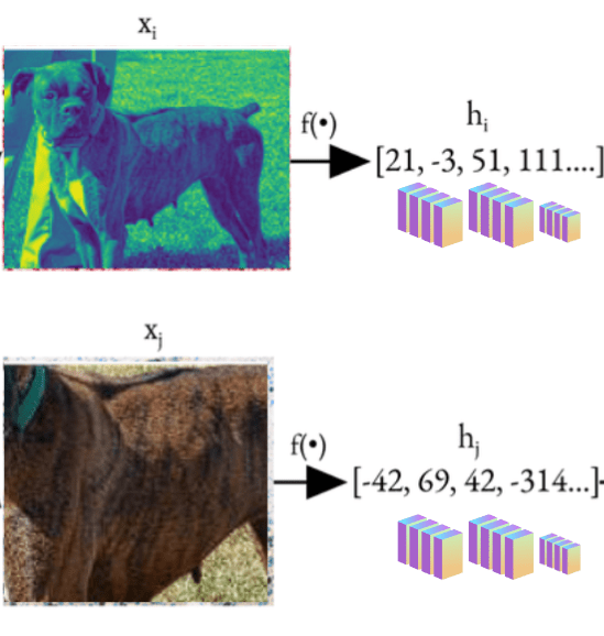
- Encode both views using the ResNet encoder to get learned representations h1 and h2.
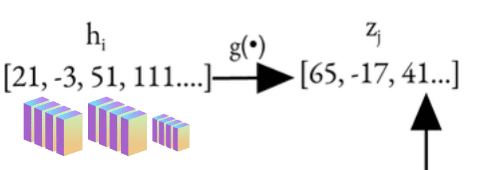
- Pass the encoded representations through the projection head to get projections z1 and z2 in the feature space.
- Compute the NT-Xent loss over all pairs (positive and negative) and then maximize the agreement between the projections in the feature space itself.
- Backpropagate gradients and update parameters using LARS Optimizer(briefed later in the article).
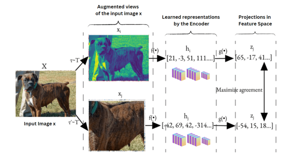
SimCLR Algorithm
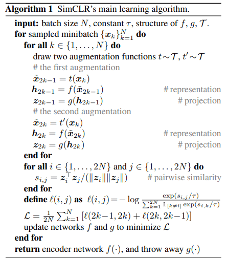
Let’s go through it in more detail –
1. Generate Augmented views
- Purpose: Generate diverse views of the same image to enforce invariance to transformations. One composition of augmentations always stands out: random cropping and random color distortion.
- Augmentation Techniques:
- Random cropping and resizing.
- Color jittering (e.g., brightness, contrast).
- Random Gaussian blur.
- Random horizontal flip.
- Loop over k∈{1,…,N}:
For each data point xk in the minibatch: Apply two augmentation functions t∼T and t′∼T to create two augmented views ![]() and
and ![]()
2. Base Encoder
- Architecture: A ResNet (e.g., ResNet-50) is used as the base encoder f(⋅).
- Function: Encodes the augmented views into latent representations:
-

- For each augmented view
 and
and  , pass it through the encoder network f to obtain the representations
  and
and  .
. - Role of Normalization:
- Batch Normalization (BN) ensures stable training by normalizing activations within mini-batches. Inconsistent statistics from local BN (e.g., each GPU using only its local mini-batch) can introduce noise, leading to degraded performance.
- Global BN is used during distributed training to maintain consistency across devices. With distributed training across multiple GPUs, the batch is split across devices. Without Global BN, the BN layers would normalize activations based on the smaller, local batch, which might not represent the full batch distribution.
-
3. Projection Head
- Architecture: A Multi-Layer Perceptron (MLP) with:
- One hidden layer.
- ReLU activation.
- Output normalized using L2 normalization.
- Purpose: Map representations
 and
and  through the projection head g to produce the projected embeddings
  and
and  into a space optimized for contrastive loss:
 ![\[z_i = g(h_i) = W^{(2)} \sigma(W^{(1)} h_i)\]](https://learnopencv.com/wp-content/ql-cache/quicklatex.com-af102df6eece9fa0a66d62c03bf1102e_l3.png)
z1 = g(h1) and z2 = g(h2)
- Reason for Projection Head:
- It improves representation quality in h by applying the contrastive loss on z.
- Key observation: a nonlinear projection is better than a linear projection (by +3%), and much better than no projection (by >10%). Even when nonlinear projection is used, the layer before the projection head, h, is still much better (>10%) than the layer after, z = g(h), which shows that the hidden layer before the projection head is a better representation than the layer after. Projection Head sacrifices some information (e.g. color, orientation) to optimize contrastive loss, making h suitable for other tasks.
4. Compute Pairwise Similarities:
- Loop over all augmented examples i, j ∈ {1,…,2N}:
- Compute the cosine similarity si,j between all pairs of embeddings:
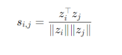
- This measures how similar two embeddings zi and zj are in the projection space.
5. Loss Function
- Contrastive Loss (NT-Xent):
- Maximizes the similarity of positive pairs z1, and z2 using cosine similarity.
- Minimizes the similarity with negative pairs (other images in the batch).

- The final loss L is averaged over all positive pairs in the batch:

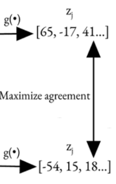
6. Optimizer
Update the encoder f and projection head g to minimize the contrastive loss L. Then, at the end of the training, discard the projection head g and use only the encoder f for downstream tasks.
- LARS (Layer-wise Adaptive Rate Scaling):
- The optimizer modifies the learning rate for each layer or parameter group adaptively, based on the magnitude of weights and gradients. Used for large batch sizes to adaptively scale learning rates for different layers with the help of trust-ratio (ensures learning rates adapt to the scale of weights and gradients). In broader terms, LARS uses layer-specific learning rates to avoid over-penalizing certain layers during optimization.
- Why LARS?
- Handles large-batch challenges and stabilizes training across layers. LARS helps SimCLR efficiently handle the gradient updates across layers when working with large-scale data and contrastive loss, which involves computing pairwise similarities.
In SimCLR, if a batch contains N images, it generates 2N views (two views per image). For each view zi, its positive pair is the other view of the same image. This means all other views (2N-2) in the batch are considered negative pairs, regardless of their actual semantic similarity. When multiple instances of the same image or class are present in the batch, this setup can result in false negatives. False negatives happen when the model incorrectly treats semantically similar views (such as different instances of the same image or class) as negative pairs, even though they should be positives.
How SimCLR addresses this problem
- Large batch size – with large batches (e.g., 4096 samples), the proportion of false negatives is minimized.
- Strong augmentations
- Projection Head – The projection head ensures that representations used for contrastive learning are mapped to a latent space optimized for the contrastive objective, which may mitigate some issues caused by false negatives.
- Hard Negative Mining – Instead of treating all other views as negatives, use a similarity threshold to include harder negatives that are dissimilar to the anchor selectively.
To address all these challenges of SimCLR, student-teacher learning-based architectures (BYOL, etc.) started getting more popular.
These constitute the theoretical foundations and explanatory framework underlying the SimCLR methodology. Moving a step forward towards BYOL (Bootstrap Your Own Latent), it will be good to understand a bit about the Student-Teacher model too.
Student-Teacher model aka Knowledge Distillation
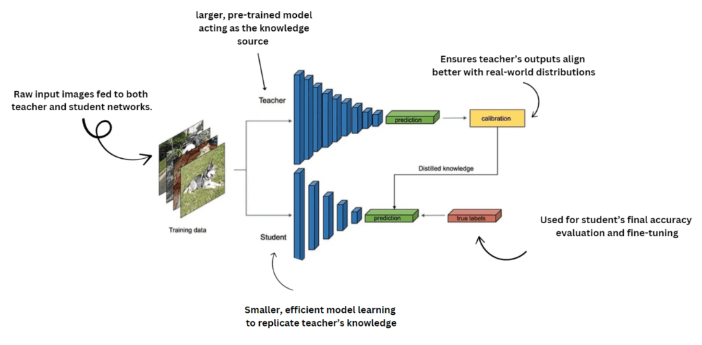
The student-teacher model became prominent with the work of Geoffrey Hinton et al. in their paper on Knowledge Distillation where –
- The Teacher network is a large, pre-trained model. It provides stable target representations from which the student network can learn. The network evolves slowly based on the student’s parameters, ensuring stability and avoiding representation collapse.
- The student network learns by mimicking the teacher’s output (soft predictions). It learns to predict the embeddings generated by the teacher.
This introduced the idea of transferring knowledge from a larger, complex teacher model to a smaller, more efficient student model.
BYOL is a true student-teacher framework where the momentum encoder acts as the teacher, providing stable targets for the student to learn from. We’ll learn more about ‘momentum-encoder’ later in this article, but first, let’s explore what BYOL is and its implementation.
BYOL (Bootstrap Your Own Latent)
BYOL is a landmark paper on the path of understanding today’s state-of-the-art foundation models such as the DINO family including DINOv2.
The term “Bootstrap” in Bootstrap Your Own Latent (BYOL) refers to the concept of self-improvement without external labels or explicit supervision. In the context of BYOL, the model “bootstraps” its learning process by improving its representations using a self-reinforcing mechanism.
BYOL is a new algorithm for self-supervised learning of image representations. While other state-of-the-art methods (like SimCLR) rely on negative pairs, BYOL achieves a new state-of-the-art without them. It iteratively bootstraps the outputs of a network to serve as targets for an enhanced representation. According to the authors of BYOL, non-reliance on negative pairs has made BYOL more robust to the choice of image augmentations. SimCLR’s authors believed that contrastive loss could focus on aligning representations based on color information alone rather than learning meaningful features, and only because of this did SimCLR fail to retain other important features (textures and shapes). However, BYOL is still more robust because even if image augmentations share the same color histogram, it is still incentivized to retain additional features in its representation.
BYOL’s overview – Starting from an augmented view of an image, BYOL trains its online network to predict the target network’s representation of another augmented view of the same image. This flow may lead to collapsed solutions (producing the same vector for all images). However, the addition of a predictor to the online network and the use of a slow-moving average of the online parameters as the target network encourages encoding more and more information within the online projection thus bootstrapping itself to better performance without any external supervision or reliance on negatives and thus eventually avoids collapsed solutions.
BYOL uses two networks – Online (student) and Target (teacher) which interact and learn from each other.
The learning loop of BYOL is as follows –
- The student network receives an input (e.g., an augmented view of an image) and learns to predict the target output produced by the teacher network, which processes another augmented view of the same input.
- By repeatedly minimizing the difference between the student’s predictions and the teacher’s targets, the student improves its latent representations.
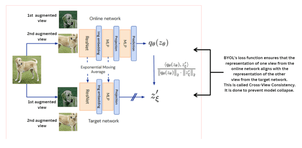
The self-reinforcing loop of BYOL is as follows –
- The online (student) network is updated using gradient descent to predict the target (produced by the teacher network).
- The teacher network is updated as a moving average of the student network, creating a stable and consistent target.
BYOL’s Architecture
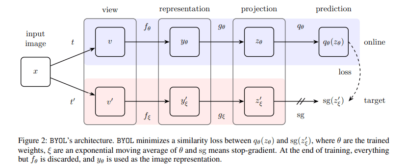
Architecture Components –
- Input image x:
- A single image is taken as input.
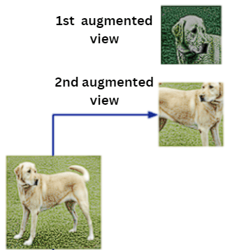
- Two augmented views of the image are generated using two independent augmentation functions t ~ T and t’ ~ T’
- These views are denoted as 𝒗 = t(x) and 𝒗’ = t’(x)
- Online Network (top pipeline):
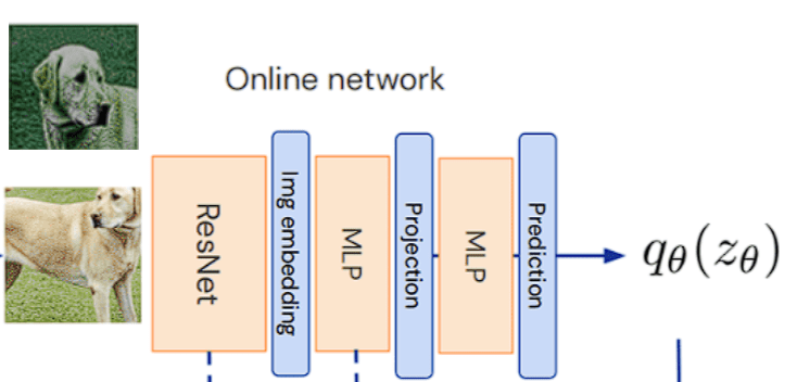
- The online network is responsible for processing one augmented view (v):
- Encoder fθ: Extracts a representation yθ = fθ(v)
- Projection Head gθ: The representation (yθ) from the encoder is passed through a Multi-Layer Perceptron (MLP) called the projection head. The structure of MLP is –
Linear Layer -> Batch-Normalization -> ReLU -> Linear Layer
We can infer from the MLP’s structure that the output of the MLP Projection Head is not Batch-normalized and this is done because Batch-Normalization at the output layer could distort the relative feature magnitudes which might interfere with the learning signal during alignment.
Maps the representation into a latent projection or to a lower-dimensional space (e.g. 2048 -> 4096 -> 256)
zθ = gθ(yθ)
- Predictor qθ: Outputs a prediction qθ(zθ), which attempts to match the target network’s output by projecting zθ into a space that aligns with the target network’s projection.
- Target Network (bottom pipeline)
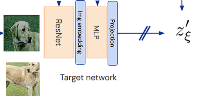
- The target network processes the second augmented view (v’):
- Encoder f𝛏: Produces a representation y𝛏 = f𝛏(v’)
- Projection Head g𝛏: Maps the representation into a latent projection
z’𝛏 = g𝛏(y𝛏)
- The target network’s weights (ξ) are exponentially moving averages (EMA) of the online network’s weights (θ):
ξ←𝜏⋅ξ+(1−𝜏)⋅θ
𝜏: Momentum coefficient, typically close to 1 (e.g., 0.99 or 0.999).
- Momentum coefficient 𝜏 controls how strongly the teacher network weights depend on the online network. Higher Momentum 𝜏 = 1.0 corresponds to the target network changing slowly and retaining past information longer while Lower Momentum 𝜏 = 0.9 helps the target network adapt more quickly to the online network.
- EMA (Exponential Moving Average) is a mathematical technique used to compute a weighted average of a quantity (here referring to online networks’s parameters) over time, giving more weight to recent values while gradually discounting older ones.
- No back-propagation is involved for parametric updates. Removal of gradients is done so that weights evolve more smoothly and consistently.
- Stop-Gradient (sg)
The online network’s gradient flow is stopped at the target network to ensure it remains stable and does not get updated during backpropagation. Without stop-gradient, the online network could attempt to “correct” the target network during training, introducing instability.
- Loss Function
- BYOL minimizes the mean squared error (MSE) between the normalized prediction (q) from the online network and the normalized projection from the target network
- This drives the online network to align its predictions with the stable outputs of the target network.

Key points to take into account
- Flow in the Online Network –
Input 𝒗 -> Encoder (fθ) -> Representation (yθ) -> Projection Head (gθ) -> Projection (zθ) -> Prediction Head (qθ) -> Prediction (qθ(zθ))
- Flow in the Target Network –
Input 𝒗 -> Encoder (f𝛏) -> Representation (y’𝛏) -> Projection Head (g𝛏) -> Target Projection (z’𝛏)
- The Target network has the same architecture as the Online network but with different weights ξ compared to the online one and those weights (ξ) are simply the exponential moving average of the online network’s weights (θ).
- The target projection (z’𝛏) serves as the stable target that the online network tries to predict.
- The target projection (z𝛏) is not updated via gradients. Instead, the target network’s parameters are updated via momentum, ensuring stability.
- While going through the research papers, if you come across terms like ResNet50(2x), ResNet(4x), or any ResNet(ɳx), it simply implies the width-multipliers which scales the number of channels in each convolutional layer ɳ times. Wider networks have more parameters and computational capacity, allowing them to capture more complex features.
BYOL’s Algorithm
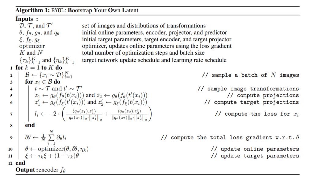
The workflow of BYOL, including its architecture components, has been outlined earlier. However, let’s take a closer look at two essential aspects: Cross-View Consistency and the Loss Function.
In BYOL, the views are swapped when computing target projections, a concept known as Cross-View Consistency. This ensures that one view’s representation from the online network aligns with the other view’s representation from the target network. Why is this crucial? Without swapping, the model might fall into the trap of trivial solutions—producing identical outputs for all inputs, effectively collapsing its ability to learn.
L2 Normalization, another key component, ensures that vector magnitudes are normalized to focus solely on their direction. This makes comparisons more meaningful, especially when aligning embeddings for the same image under different augmentations. BYOL compares these normalized embeddings using cosine similarity, scaled by -2. This scaling keeps the loss function’s range optimizer-friendly and ensures larger gradients, enabling faster and more decisive weight updates. Think of it as taking bigger steps toward the learning goal.
Interesting Insights About the BYOL Framework
Does BYOL Need Batch Statistics?
Initially, it was believed that Batch Normalization (BN) was critical for BYOL to prevent collapse. The reasoning? BN was thought to enforce dependencies across batches, introducing an Implicit Contrastive Effect—aligning representations of positives while subtly repelling negatives.
To test this, researchers replaced BN with a batch-independent normalization scheme:
- Group Normalization (GN): Normalizes data within smaller groups of channels, making it independent of batch size.
- Weight Standardization (WS): Standardizes the weights of the neural network instead of normalizing activations.
Surprisingly, this adjustment didn’t hurt performance. In fact:
- Vanilla BYOL (with BN): 73.9% top-1 accuracy on ImageNet.
- BYOL with GN + WS: 74.3% top-1 accuracy.
This result proved that batch statistics aren’t essential for BYOL to learn meaningful representations.
What Happens Without Any Batch Normalization?
Removing BN entirely from BYOL caused a dramatic performance drop to random levels—the model failed to learn anything useful. In contrast, SimCLR, another contrastive learning method, continued to perform reasonably well even without BN.
This led to an intriguing hypothesis: BN might introduce a Negative Contrastive Effect in BYOL. The hypothesis gained more weight when researchers observed differing behaviors between BYOL and SimCLR with Layer Normalization (LN) replacing BN.
- SimCLR’s performance stayed stable.
- BYOL’s performance dropped significantly.
Why does BN matter for BYOL?
It acts as a stabilizer during training, especially with poor initialization. Here’s a relatable analogy: Imagine BYOL as a teacher-student duo. The teacher updates their notes based on the student’s progress. If the student starts with bad notes (poor initialization), both struggle without an external stabilizer like BN to keep them on track.
What Makes BYOL Robust?
Despite its dependence on stabilizers like BN, BYOL’s architecture and training dynamics give it unique robustness. Features like:
- Momentum-based updates,
- Asymmetric online and target networks,
allow BYOL to excel at self-supervised representation learning even in challenging setups.
This blend of clever design choices ensures BYOL continues to shine as a cutting-edge framework in contrastive learning.
Key differences between SimCLR and BYOL

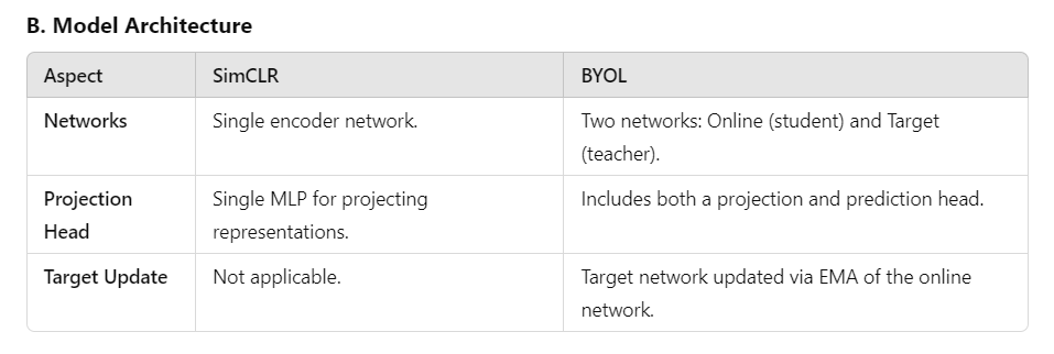


BYOL Implementation code
Now that we’ve explored the theoretical aspects of BYOL, it’s time to get our hands dirty with some implementation! In this section, we’ll train BYOL from scratch on the CIFAR-10 dataset and later use transfer learning using the pre-trained BYOL on another dataset, STL-10.
However, we won’t dive into every line of code here. Instead, we’ll focus on the most important and interesting parts of the implementation. Don’t worry—you can access and download the complete code explicitly through the links provided in this article.
So, let’s jump into the exciting journey of implementing BYOL and uncover its practical magic!
- Gaussian Blur Implementation
- Gaussian Blur to prevent the network from overfitting to specific high-frequency details (edges, textures, etc.).
- groups = 3 – channel-wise blurring because it prevents color bleeding across channels which could distort the image
- randomness in Sigma ensures two different augmented views are different but they are related too on the other hand
- Transformations
- Random cropping and resizing to fixed resolution along with Gaussian Blur
- Multi-View Data Injector
- Consistent flip to ensure the same flipping behavior is applied to all augmented views.
from torchvision.transforms import transforms
class MultiViewDataInjector(object):
    def __init__(self, *args):
        self.transforms = args[0]
        self.random_flip = transforms.RandomHorizontalFlip()

    def __call__(self, sample, *with_consistent_flipping):
        if with_consistent_flipping:
            sample = self.random_flip(sample)
        output = [transform(sample) for transform in self.transforms]
        return output
- MLP-Base
Creates the Latent Space from the Encoder.
from torch import nn
class MLPHead(nn.Module):
    def __init__(self, in_channels, mlp_hidden_size, projection_size):
        super(MLPHead, self).__init__()

        self.net = nn.Sequential(
            nn.Linear(in_channels, mlp_hidden_size),
            nn.BatchNorm1d(mlp_hidden_size),
            nn.ReLU(inplace=True),
            nn.Linear(mlp_hidden_size, projection_size)
        )

    def forward(self, x):[sc name="subscribe"]
        return self.net(x)
- SkeletonNet
Encompasses MLP-BASE for Latent Space creation and uses ResNet18 to learn feature representations
class SkeletonNet(nn.Module):
    def __init__(self,Hid,Proj):
        super(SkeletonNet,self).__init__()
        Resnet = torchvision.models.resnet18(pretrained=False)
        self.Encoder = torch.nn.Sequential(*list(Resnet.children())[:-1])
        self.Proj = MLP_Base(Resnet.fc.in_features,Hid,Proj)
    def forward(self,Input):
        Enc_Out = self.Encoder(Input)
        Enc_Out = Enc_Out.view(Enc_Out.size(0),Enc_Out.size(1))
        Final = self.Proj(Enc_Out)
        return Final
- Training Class (BYOL class) –
- Cross-view Consistency as explained above in this article
- Usage of L2-normalized kernels so that convolutions don’t introduce brightness or intensity.
def TrainLoop(self,View1,View2):
        Pred1 = self.Predictor(self.Online_Net(View1))
        Pred2 = self.Predictor(self.Online_Net(View2))
        with torch.no_grad():
            Target2 = self.Target_Net(View1)
            Target1 = self.Target_Net(View2)
        Loss_Calc = self.Loss(Pred1,Target1) + self.Loss(Pred2,Target2)
        return Loss_Calc.mean()
    def Train(self,Trainset):
        TrainLoader = torch.utils.data.DataLoader(Trainset,batch_size=self.Batch_Size,drop_last=False,shuffle=True)
        self.Init_Target_Network()
        for Epoch in range(self.Epochs):
          Loss_Count = 0.0
          print("Epoch {}".format(Epoch))
          for (View_1,View_2),_ in tqdm(TrainLoader):
              View_1 = View_1.to(self.Device)
              View_2 = View_2.to(self.Device)
              Loss = self.TrainLoop(View_1,View_2)
              Loss_Count += Loss.item()
              self.Optim.zero_grad()
              Loss.backward()
              self.Optim.step()
              self.Update_Target_Params()
          Epoch_Loss = Loss_Count/len(TrainLoader)
          print("Epoch{} Loss:{} : ".format(Epoch,Epoch_Loss))
After BYOL pretraining on the CIFAR-10 dataset, we have to look into the general transfer-learning (without much data augmentations and optimizations) of pre-trained BYOL on the STL-10 dataset. You can incorporate more transformations for better fine-tuning. The below snippets will look into our objective of fine-tuning the pre-trained BYOL.
- Downloading the dataset
device = 'cpu' #'cuda' if torch.cuda.is_available() else 'cpu'
encoder = ResNet18(**config['network'])
output_feature_dim = encoder.projetion.net[0].in_features
train_dataset = datasets.STL10('./data', split='train', download=True,
                               transform=data_transforms)

test_dataset = datasets.STL10('./data', split='test', download=False,
                               transform=data_transforms)
- Loading pre-trained BYOL’s parameters
#load pre-trained parameters
load_params = torch.load(os.path.join('./Models/BYOL.pth'),
                         map_location=torch.device(torch.device(device)))
[sc name="subscribe"]
if 'online_network_state_dict' in load_params:
    encoder.load_state_dict(load_params['online_network_state_dict'])
    print("Parameters successfully loaded.")

# remove the projection head
encoder = torch.nn.Sequential(*list(encoder.children())[:-1])
encoder = encoder.to(device)
- Training and Testing loop along with optimization –
for epoch in range(500):
    epoch_loss = 0
    logreg.train()
#     train_acc = []
    for x, y in train_loader:

        x = x.to(device)
        y = y.to(device)

        # zero the parameter gradients
        optimizer.zero_grad()

        logits = logreg(x)
        predictions = torch.argmax(logits, dim=1)

        loss = criterion(logits, y)

        loss.backward()
        optimizer.step()

        epoch_loss += loss.item()

    train_losses.append(epoch_loss / len(train_loader))

    # scheduler.step()

    if epoch % eval_every_n_epochs == 0:
        logreg.eval()
        correct = 0
        total = 0
        for x, y in test_loader:
            x = x.to(device)
            y = y.to(device)

            logits = logreg(x)
            predictions = torch.argmax(logits, dim=1)

            total += y.size(0)
            correct += (predictions == y).sum().item()

        acc = 100 * correct / total
        test_accuracies.append(acc)
        print(f"Epoch {epoch}, Testing accuracy: {acc:.2f}%")
This was all about implementing BYOL and then using its learned representations for downstream tasks.
Key Takeaways
- Contrastive Learning promises to bridge supervised and unsupervised learning by teaching models to distinguish similarities and differences, enabling powerful self-supervised systems.
- While SimCLR thrives on negative samples and large batches to refine representations, BYOL stands out with its momentum-based student-teacher framework, eliminating the need for negatives and proving more robust to augmentations.
- Innovations like LARS optimization for SimCLR, momentum updates, and batch normalization in the case of BYOL have played a pivotal role in stabilizing and enhancing representation learning. Though batch statistics aren’t essential for BYOL to learn meaningful representations, still they act as a savior in case of poor initializations.
Conclusion
This article explores the transformative field of Contrastive Learning, diving into its evolution, core concepts, and implementation through frameworks like SimCLR and BYOL. From SimCLR’s reliance on negative samples to BYOL’s groundbreaking momentum-based updates without negatives, we examined the practicalities of their training algorithms, architectural nuances, loss functions, and evaluation techniques with detailed examples and explanations.
As the field evolves, methods like MoCo, SimSiam, and CLIP push boundaries, making contrastive learning more efficient, adaptable, and multimodal. The journey from handcrafted labels to self-supervised representation learning signifies a fundamental shift toward AI systems that learn organically from their environment. Contrastive Learning, led by frameworks like SimCLR and BYOL, is not just a methodology but a paradigm, shaping the future of machine learning with its potential to create truly intelligent and adaptable systems.
References
- Contrastive Divergence
- Instance-level Discrimination
- Supervised Contrastive Learning
- SimCLR
- Distilling the Knowledge in a Neural Network
- Momentum Contrast for Unsupervised Visual Representation Learning
- BYOL
- BYOL doesn’t need batch-statistics
- Understanding Self-Supervised Learning Dynamics without Contrastive Pairs
- BYOL official source code
- BYOL’s implementation reference source code




100K+ Learners
Join Free OpenCV Bootcamp3 Hours of Learning