Image classification is used to solve several Computer Vision problems; right from medical diagnoses, to surveillance systems, on to monitoring agricultural farms. There are innumerable possibilities to explore using Image Classification.
If you have completed the basic courses on Computer Vision, you are familiar with the tasks and routines involved in Image Classification tasks. Want to know more?
Image Classification tasks follow a standard flow – where you pass an image to a deep learning model and it outcomes the class or the label of the object present.
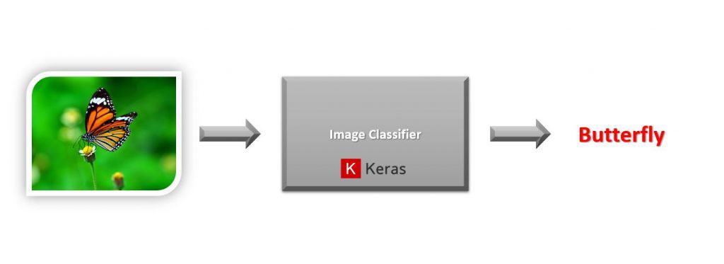
While learning Computer Vision, most often a project that would be equivalent to your first hello world project, will most likely be an image classifier. You attempt to solve something like the digit recognition on MNIST Digits dataset or maybe the Cats and Dog Classification problem.
The Deep Learning wave started in 2012. It was primarily due to Alexnet, a Convolutional Neural Network (CNN) image classifier.
Image Classifiers not only have a big place in industrial applications but also are a very natural resource to learn about Computer Vision and CNNs.
The most popular frameworks for creating image classifiers are either Keras (a wrapper over Tensorflow) or Pytorch. Even if you have never coded a Neural network, with these libraries you can actually create and train a decent deep learning model with just a few lines of code. You need not build anything from scratch, simply use the inbuilt features, that too in a matter of minutes!
Another important problem in Computer Vision, similar to classification, is Object Detection, where you pass in an image to a Deep Learning model and you get class labels and also some bounding box coordinates, telling you where exactly the object is present in the image.
This extra location information can be really useful in real-life applications such as self-driving cars. In such applications you need to know where exactly the other cars are present on the road.

You might start thinking now: Can you create an Object Detector in Keras?
Of course, you can; but you may have to write a lot of code. You would also need a lot of prior knowledge to be able to train the Object Detector correctly. It’s also really easy to make mistakes and the hardest part is to debug the code in case of errors.
If you still have doubts then just take a look at this Official Keras code for creating and training a custom RetinaNet detector.
Fortunately, if you want to train an Object Detector, you actually won’t need to code everything in Keras. The TensorFlow team provides you with Tensorflow Object Detection (TFOD) API – a high-level API for TensorFlow built specifically to make it easier to train Object Detection models.
Usually, beginners get comfortable with creating classifiers and take time to move to TFOD API to create detection models because they face installation problems, computation requirements, confusing steps, lots of scripts to run, etc.
From a beginner’s perspective, these are all valid issues but I would say the TFOD API has gotten a lot better in the past few months. Especially with TF 2.0 support, it comes with many models, better integration with Keras, and much more.
Still, a fact remains that for early practitioners, it can be a bit intimidating to explore this API.
At this stage, you might start wondering: Why follow such a complicated model and features? Can’t we simply modify our classifiers so they perform detection as well?
Well, actually YOU CAN.
How to make Classifiers perform detection?
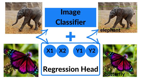
The answer would be to create a multi-output classification network with two output branches. One branch can output class labels and the second one can output your bounding box coordinates.
If you are not familiar with Multi-Output Models, visualize them to be types of architecture that can have multiple branches inside the same network to output different things.
Still feel confused about how a multi-output model can be created for detection purposes? Don’t worry, we are here to help you. You may want to watch this lecture on Object Localization by Andrew Ng from his deepleaning.ai specialization. He explains the full concept in a really simple and clear manner.
You might ask if creating detectors this way is really easy and effective, then why don’t more people do it this way?
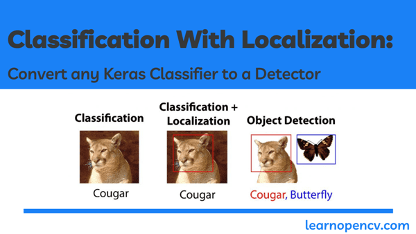
Well, there’s a catch. Simply speaking, the approach I’ve described above is not exactly Object Detection. It’s actually called Classification with Localization.
Why is it so?
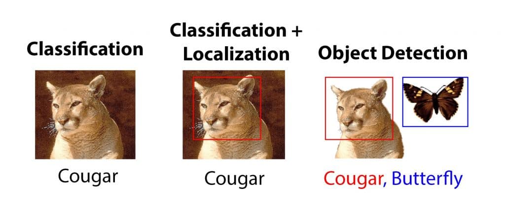
In normal Object Detection, you can detect multiple objects in a single image. On the other hand, classification with localization setup is limited to detecting only one object per image. (You could theoretically include more boxes, but your network performance will be really poor).
Here’s an image that explains the difference.
Classification With Localization (Keras Code):
Now that we have understood what we want to achieve, let’s start with the code. Make sure to download the code from the Download Section.
Here’s our outline of the pipeline:
- Step 1: Downloading the Detection Dataset
- Step 2: Perform Data Augmentation with imgaug library
- Step 3: Preprocess the Dataset
- Step 4: Visualize the Data with its Annotations
- Step 5: Split the Data into Train and Validation Set
- Step 6: Construct the Multi-Output Model
- Step 7: Compile & Train the Model
- Step 8: Plot Model’s Loss & Accuracy Curves
- Step 9: Test your model on New Images
Step 1: Downloading the Detection Dataset
Let’s start by downloading the dataset. We have extracted a subset of the CALTECH-101 dataset and created a dataset which contains images for only 3 classes, namely elephant, butterfly, and cougar-face. The class labels and bounding box coordinates for each image are present in .MAT (Matlab) format.
After downloading the data, you will need to extract it.
# Download the dataset
!wget -O CALTECH.zip https://zenodo.org/record/4126613/files/CALTECH.zip?download=1

# Extract all the contents of zip file in current directory
with ZipFile('CALTECH.zip', 'r') as zipObj:
   zipObj.extractall()
Step 2: Perform Data Augmentation with imgaug library
Data Augmentation is a very useful technique to expand a dataset and make a model generalize better.
There are many types of augmentations we can perform on images. Normally when you’re dealing with an image classification problem, you can do augmentation with the Keras built-in function –
tf.keras.preprocessing.image.ImageDataGenerator
Note: Unfortunately, we can’t use the ImageDataGenerator in this notebook!
Why not?
We will not be able to use it in augmentation because we employ techniques like shift, rotation, shear, crop, zoom, etc. All these techniques will fundamentally change the image but when the images change the corresponding bounding box coordinates should also change. Since the Keras augmentation function only modifies the image and not the box coordinates so it’s a really bad idea to use the default augmentation function.
So what can we do?
Well, we have 3 options.
- Use the Keras default augmentation module but use augmentations that do not change the image spatially. e.g. centering, normalization, whitening, etc.
- Create our own custom augmentation functions which modify the images as well as the bounding boxes.
- Use a library like imgaug, which allows you to augment images and bounding box locations.
Now, which one should we use?
Option 1 is by far the least effective – if you’re not spatially modifying the image then you don’t have many options.
If you go with Option 2 then you would need to write a lot of boilerplate code and deal with bugs.
For this notebook, I went with option 3, which is the most effective option. imgaug library will allow us to do a number of augmentations. The best part being that these changes will also be applied to the respective bounding boxes.
With imgaug we will apply 7 different types of augmentations to our dataset:
- Rescaling the image
- Rotating the image
- Shifting the image
- Flipping the image
- Changing the brightness
- Blurring to the image
- Adding Noise to the image
You can look at imgaug docs here.
The code we have written will randomly use any 3 of these augmentations on each image
The data augmentation scheme performed here is a modified version of the one by Asset Karazhay explained in this post.
Convert MAT Labels into CSV
To perform data augmentation we first have to convert our labels into a CSV format. This helps the imgaug library to use the labels to augment the images easily as well as their bounding boxes.
Function to Extract MAT attributes:
The CALTECH-101 dataset comes in the form of MATLAB files. Since we’ll be modifying our classifier to do detection we need the annotations in a more familiar format. So what we’ll do is create a function to extract the class label and the bounding box coordinates (x1, y1, x2, y2) from each MAT File. We will also extract the name of the image so we can associate each MAT file with its corresponding image.
def extract_mat_contents(annot_directory, image_dir):

        # Create MAT Parser
        mat = scipy.io.loadmat(annot_directory)

        # Get the height and width for our image
        height, width = cv2.imread(image_dir).shape[:2]

        # Get the bounding box co-ordinates
        x1, y2, y1, x2 = tuple(map(tuple, mat['box_coord']))[0]

        # We Split the image Directory passed in the method and choose the index
        # Of the Folders name which is the same as it's class
        class_name = image_dir.split('/')[2]

        filename = '/'.join(image_dir.split('/')[-2:])

        # Return the extracted attributes
        return filename,  width, height, class_name, x1,y1,x2,y2
The function above will be used in the function below to go through the image and annotation directories and to extract their information such as:
- Height
- Width
- Bounding box coordinates
- Class
Once extracted, this information will be stored in a pandas dataframe which helps us use it with imgaug to perform augmentations.
# Function to convert MAT files to CSV
def mat_to_csv(annot_directory, image_directory, classes_folders):

  # List containing all our attributes regarding each image
  mat_list = []

  # We loop our each class and its labels one by one to preprocess and augment
  for class_folder in classes_folders:

    # Set our images and annotations directory
    image_dir = os.path.join(image_directory, class_folder)
    annot_dir = os.path.join(annot_directory, class_folder)

    # Get each file in the image and annotation directory
    mat_files = sorted(os.listdir(annot_dir))
    img_files = sorted(os.listdir(image_dir))

    # Loop over each of the image and its label
    for mat, image_file in zip(mat_files, img_files):

      # Full mat path
      mat_path = os.path.join(annot_dir, mat)

      # Full path Image
      img_path = os.path.join(image_dir, image_file)

      # Get Attributes for each image
      value = extract_mat_contents(mat_path, img_path)

      # Append the attributes to the mat_list
      mat_list.append(value)

  # Columns for Pandas DataFrame
  column_name = ['filename', 'width', 'height', 'class', 'xmin', 'ymin',
                 'xmax', 'ymax']

  # Create the DataFrame from mat_list
  mat_df = pd.DataFrame(mat_list, columns=column_name)

  # Return the dataframe
  return mat_df

# The Classes we will use for our training
classes_list = sorted(['butterfly',  'cougar_face', 'elephant'])

# Set our images and annotations directory
image_directory = 'CALTECH/CALTECH_Dataset'
annot_directory = 'CALTECH/CALTECH_Annotations'

# Run the function to convert all the MAT files to a Pandas DataFrame
labels_df = mat_to_csv(annot_directory, image_directory, classes_list)

# Saving the Pandas DataFrame as CSV File
labels_df.to_csv(('labels.csv'), index=None)
Now that we have the data ready in the required format, let’s proceed to perform the augmentations.
In this step, we will create a helper function which will convert imagaug’s bounding box objects to panda’s dataframe.
# Function to convert bounding box image into DataFrame
def bounding_boxes_to_df(bounding_boxes_object):

    # Convert Bounding Boxes Object to Array
    bounding_boxes_array = bounding_boxes_object.to_xyxy_array()

    # Convert the array into DataFrame
    df_bounding_boxes = pd.DataFrame(bounding_boxes_array,columns=['xmin', 'ymin', 'xmax', 'ymax'])

    # Return the DataFrame
    return df_bounding_boxes
Initialize the Augmentations
Initialize the imgaug library with the augmentations we are going to use with the images. imgaug selects n random augmentations from the list below and applies it to an image. For every image, a new random combination of augmentation is used. You can set this value of n below as needed. Here, I’m setting it to 2.
# Define all the Augmentations you want to apply to your dataset
# We're setting random `n` agumentations to 2.
image_augmentations = iaa.SomeOf( 2,
    [
    # Scale the Images
    iaa.Affine(scale=(0.5, 1.5)),

    # Rotate the Images
    iaa.Affine(rotate=(-60, 60)),

    # Shift the Image
    iaa.Affine(translate_percent={"x":(-0.3, 0.3),"y":(-0.3, 0.3)}),

    # Flip the Image
    iaa.Fliplr(1),

    # Increase or decrease the brightness
    iaa.Multiply((0.5, 1.5)),

    # Add Gaussian Blur
    iaa.GaussianBlur(sigma=(1.0, 3.0)),

    # Add Gaussian Noise
    iaa.AdditiveGaussianNoise(scale=(0.03*255, 0.05*255))

])
As you can see we are not only adding different types of augmentations but also setting some range for each type of augmentation. You can change these values, for more information on augmentation options in imgaug, refer to this.
Create a Function to Apply Augmentations
This function will finally perform the image augmentations to both images and bounding boxes. It will read the labels dataframe we created earlier to obtain the bounding box information for each image and as it augments the image. Then it will also edit the bounding box coordinates so the coordinates remain true even after image is processed.
def image_aug(df, images_path, aug_images_path, augmentor, multiple = 3):

    # Fill this DataFrame with image attributes
    augmentations_df = pd.DataFrame(
        columns=['filename','width','height','class', 'xmin', 'ymin', 'xmax','ymax'])

    # Group the data by filenames
    grouped_df = df.groupby('filename')

    # Create the directory for all augmentated images
    if not os.path.exists(aug_images_path):
      os.mkdir(aug_images_path)

    # Create directories for each class of augmentated images
    for folder in df['class'].unique():
      if not os.path.exists(os.path.join(aug_images_path, folder)):
        os.mkdir(os.path.join(aug_images_path, folder))

    for i in range(multiple):

      # Post Fix we add to the each different augmentation of one image
      image_postfix = str(i)

      # Loop to perform the augmentations
      for filename in df['filename'].unique():

        augmented_path = os.path.join(aug_images_path, filename)+image_postfix+'.jpg'

        # Take one image at a time with its information
        single_image = grouped_df.get_group(filename)
        single_image = single_image.reset_index()
        single_image = single_image.drop(['index'], axis=1)

        # Read the image
        image = imageio.imread(os.path.join(images_path, filename))

        # Get bounding box
        bounding_box_array = single_image.drop(['filename', 'width', 'height','class'], axis=1).values

        # Give the bounding box to imgaug library
        bounding_box = BoundingBoxesOnImage.from_xyxy_array(bounding_box_array, shape=image.shape)

        # Perform random 2 Augmentations
        image_aug, bounding_box_aug = augmentor(image=image,bounding_boxes=bounding_box)

        # Discard the the bounding box going out the image completely
        bounding_box_aug = bounding_box_aug.remove_out_of_image()

        # Clip the bounding box that are only partially out of th image
        bounding_box_aug = bounding_box_aug.clip_out_of_image()

        # Get rid of the the image if bounding box was discarded
        if re.findall('Image...', str(bounding_box_aug)) == ['Image([]']:
            pass

        else:

          # Create the augmented image file
          imageio.imwrite(augmented_path, image_aug)

          # Update the image width and height after augmentation
          info_df = single_image.drop(['xmin', 'ymin', 'xmax', 'ymax'], axis=1)
          for index, _ in info_df.iterrows():
              info_df.at[index, 'width'] = image_aug.shape[1]
              info_df.at[index, 'height'] = image_aug.shape[0]

          # Add the prefix to each image to differentiate if required
          info_df['filename'] = info_df['filename'].apply(lambda x: x + image_postfix + '.jpg')

          # Create the augmented bounding boxes dataframe
          bounding_box_df = bounding_boxes_to_df(bounding_box_aug)

          # Concatenate the filenames, height, width and bounding boxes
          aug_df = pd.concat([info_df, bounding_box_df], axis=1)

          # Add all the information to augmentations_df we initialized above
          augmentations_df = pd.concat([augmentations_df, aug_df])

    # Remove index
    augmentations_df = augmentations_df.reset_index()
    augmentations_df = augmentations_df.drop(['index'], axis=1)

    # Return the Dataframe
    return augmentations_df

augmented_images_df = image_aug(labels_df, image_directory, 'aug_images',
                                image_augmentations)
Apply the function above for augmentation.
augmented_images_df = augmented_images_df.sort_values('filename', ignore_index= True)
augmented_images_df.to_csv('aug.csv')

# Check Dataset Size
print('Our total dataset Size before the augmentations was: ', len(labels_df))
print('Our total dataset Size after the augmentations is: ', len(augmented_images_df))
Our total dataset size before the augmentations was:  218
Our total dataset size after the augmentations is:  654
Step 3: Preprocess the Dataset
Now we will start converting class labels to one-hot encoded vectors and the bounding boxes will be scaled to range 0-1 because it’s easier for the network to predict values in a fixed range for each image. Plus we will be using the sigmoid activation function for the localization/regression head and sigmoid outputs values between 0-1.
We will also preprocess the image by resizing it to a fixed size, converting it to RGB channel format, and normalizing it by dividing it by 255.0. This will help the network in training.
def preprocess_dataset(image_folder, classes_list, df, image_size = 300,):

  # Lists that will contain the whole dataset
  labels = []
  boxes = []
  img_list = []

  # Get height and width of each image in the datafame
  h = df['height']
  w = df['width']

  # Create a copy of the labels in the dataframe
  labels = list(df['class'])

  # Create a copy of the bounding box values and also normalize them
  for x1, y1, x2, y2 in zip(list(df['xmin']/w), list(df['ymin']/h),list(df['xmax']/w), list(df['ymax']/h)):

    arr = [x1, y1, x2, y2]
    boxes.append(arr)

  # We loop over each class and its labels
  for class_folder in classes_list:

    # Set our images directory
    image_dir = os.path.join(image_folder, class_folder)

    # Annotation and Image files
    img_files = sorted(os.listdir(image_dir))

    # Loop over each of the image and its label
    for image_file in img_files:

      # Full path Image
      img_path = os.path.join(image_dir, image_file)

      # Read the image
      img  = cv2.imread(img_path)

      # Resize all images to a fix size
      image = cv2.resize(img, (image_size, image_size))

      # Convert the image from BGR to RGB as NasNetMobile was trained on RGB images
      image = cv2.cvtColor(image, cv2.COLOR_BGR2RGB)

      # Normalize the image by dividing it by 255.0
      image = image.astype("float") / 255.0

      # Append it to the list of images
      img_list.append(image)

  return labels, boxes, img_list
Now call the preprocessing function.
# All images will resized to 300, 300
image_size = 300

# Get Augmented images and bounding boxes
labels, boxes, img_list = preprocess_dataset('aug_images', classes_list, augmented_images_df)
We will shuffle the data after preprocessing is completed.
# Convert labels to integers, then one hot encode them
label_encoder = LabelEncoder()
integer_labels = label_encoder.fit_transform(labels)
onehot_labels = to_categorical(integer_labels)

# Now we need to shuffle the data, so zip all lists and shuffle
combined_list = list(zip(img_list, boxes, onehot_labels))
random.shuffle(combined_list)

# Extract back the contents of each list
img_list, boxes, onehot_labels = zip(*combined_list)

print('All Done')
Step 4: Visualize the Data with its Annotations
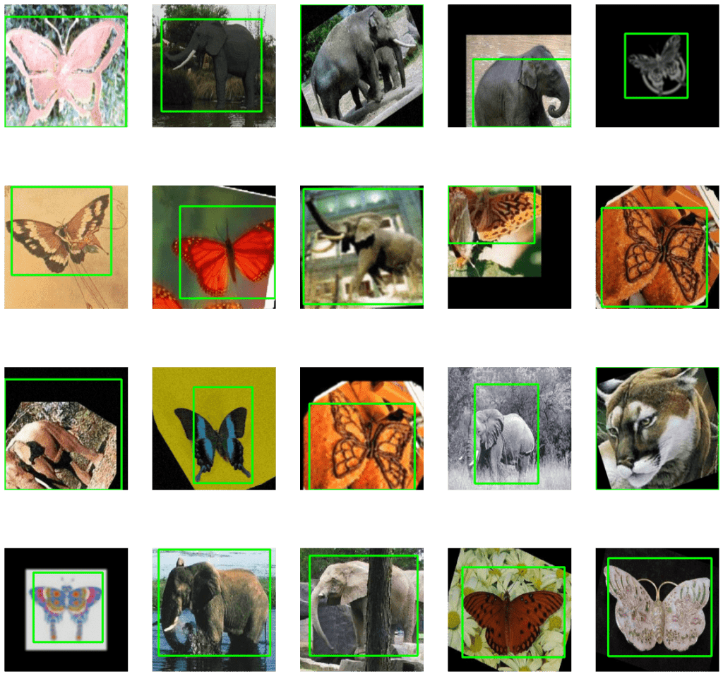
Here we will pick some random images from each class and draw the associated bounding boxes over it. This way you’ll be able to visualize the data and make sure that your preprocessing steps were performed correctly.
# Create a Matplotlib figure
plt.figure(figsize=(20,20));

# Generate a random sample of images each time the cell is run
random_range = random.sample(range(1, len(img_list)), 20)

for iteration, i in enumerate(random_range, 1):

    # Bounding box of each image
    a1, b1, a2, b2 = boxes[i];

    # Rescaling the boundig box values to match the image size
    x1 = a1 * image_size
    x2 = a2 * image_size
    y1 = b1 * image_size
    y2 = b2 * image_size

    # The image to visualize
    image = img_list[i]

    # Draw bounding boxes on the image
    cv2.rectangle(image, (int(x1),int(y1)),
          (int(x2),int(y2)),(0,255,0),3);

    # Clip the values to 0-1 and draw the sample of images
    image = np.clip(img_list[i], 0, 1)
    plt.subplot(4, 5, iteration);
    plt.imshow(image);
    plt.axis('off');
Step 5: Split the Data into Train and Validation Set
Now we would have 3 lists; one list containing all images, the second one contains all class labels in one-hot encoded format, and the third one list contains scaled bounding box coordinates. Let’s split our data to create a training and validation set. It’s important to shuffle your data before the split which we have already done.
# Split the data of images, labels and their annotations
train_images, val_images, train_labels, \
val_labels, train_boxes, val_boxes = train_test_split( np.array(img_list),
                np.array(onehot_labels), np.array(boxes), test_size = 0.1,random_state = 43)

print('Total Training Images: {}, Total Test Images: {}'.format(
    len(train_images),
    len(val_images)
    ))
Total Training Images: 392, Total Test Images: 44
Step 6: Construct the Multi-Output Model
Now it’s time to create our Multi-Output model. We won’t be training from scratch but we will use transfer learning. The model we will use is NasnetMobile. This is a really efficient model with a good balance of speed and accuracy, It was created through Neural Architecture Search (NAS) which is an emerging field of AutoML.
We’ll first download the model but exclude the top since we’ll be adding our own custom top.
# Load the NasNetMobile Model, make sure to exclude the top for transfer learning
N_mobile = tf.keras.applications.NASNetMobile( input_tensor = Input(
    shape=(image_size, image_size, 3)),
    include_top=False,
    weights='imagenet'
    )
# Let's create a function that will construct our model
def create_model(no_of_classes):

    # Freeze the whole model
    N_mobile.trainable = False

    # Start by taking the output feature maps from NASNETMobile
    base_model_output = N_mobile.output

    # Convert to a single-dimensional vector by Global Average Pooling.

    # We could also use Flatten()(x) but GAP is more effective, it reduces
    # Parameters and controls overfitting.
    flattened_output = GlobalAveragePooling2D()(base_model_output)

    # Create our Classification Head, final layer contains
    # Ouput units = no. classes
    class_prediction = Dense(256, activation="relu")(flattened_output)
    class_prediction = Dense(128, activation="relu")(class_prediction )
    class_prediction = Dropout(0.2)(class_prediction)
    class_prediction = Dense(64, activation="relu")(class_prediction)
    class_prediction = Dropout(0.2)(class_prediction )
    class_prediction = Dense(32, activation="relu")(class_prediction)
    class_prediction = Dense(no_of_classes, activation='softmax',name="class_output")(class_prediction)

    # Create Our Localization Head, final layer contains 4 nodes for x1,y1,x2,y2
    # Respectively.
    box_output = Dense(256, activation="relu")(flattened_output)
    box_output = Dense(128, activation="relu")(box_output)
    box_output = Dropout(0.2)(box_output )

    box_output = Dense(64, activation="relu")(box_output)
    box_output = Dropout(0.2)(box_output )

    box_output = Dense(32, activation="relu")(box_output)
    box_predictions = Dense(4, activation='sigmoid',
                            name= "box_output")(box_output)

    # Now combine the two heads
    model = Model(inputs=N_mobile.input, outputs= [box_predictions, class_prediction])

    return model

# Create the model for 3 classes, Elephant, Butterfly, Cougar-Face
model = create_model(3)
print("Model Created")
Check Model’s Structure:
Using the plot_model function you can check the structure of the final model. This is really helpful when you are creating a complex network and you want to make sure you have constructed the network correctly.
plot_model(model, to_file='model_plot.png', show_shapes=True, show_layer_names=True)
When you run the above code, you will get the graph image below. This plot will also be saved to your disk as model_plot.png.
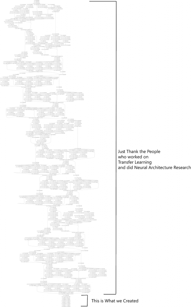
Don’t worry about deciphering the whole network. We started the deep learning explosion with networks like Alexnet and then kept innovating with models like VGG, inception, Resnet, and other complex residual architectures every year. We also innovated and created new layer operations like BatchNormalization to combat overfitting and achieve faster training, and so created Dropout, Separable Convolutions, and many more.
Today we’re living in a time where architectures created from Neural Architecture Search achieve state of the art levels in accuracy and performance.
Here’s the expanded part of the graph that we created.
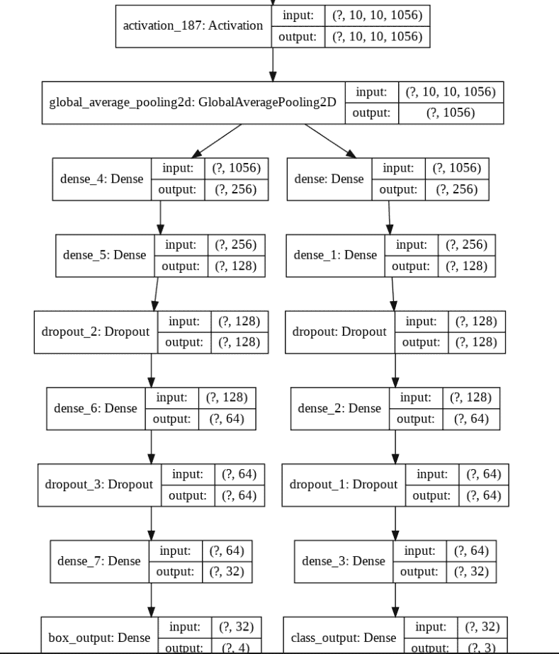
So upon looking at the above graph we can say that the network is structured as intended. We are now ready to proceed to the next step.
Step 7: Compile & Train the Model
Now here are a couple of things that you need to do before we compile and train the model. In case of a single output model you just have to define a loss, a metric, and an optimizer and compile the model. Since we’re dealing with a multi-output model that outputs two totally different things, we need to use separate loss and separate metrics for each these output branches.
Remember when we were creating the model we actually assigned names to our two output branches. By doing so, we can easily refer to the name of an output branch and then assign it a specific loss or metric – just like a python dictionary.
# Here for each head we will define a different loss, we will define it
# Like a dictionary.

# For classification we will have cateogirical crossentropy
# For the bouding boxes we will have mean squared error
losses = {
    "box_output": "mean_squared_error",
    "class_output": "categorical_crossentropy"
    }

# Here you can give more or less weightage to each loss.

# If you think that detection is harder then the classification then you can
# Try assinging it more weight
loss_weights = {
    "box_output": 1.0,
    "class_output": 1.0
    }

# Set the Metrics
# For the class labels we want to know the Accuracy
# And for the bounding boxes we need to know the Mean squared error
metrics = {
    'class_output': 'accuracy',
    'box_output':  'mse'
    }

# We will be using early stopping to stop the model if total val loss does not
# Decrease by 0.001 in 40 epochs
stop = EarlyStopping(monitor = "val_loss", min_delta = 0.0001, patience = 40,
                    restore_best_weights = True
                     )

# Change the learning rate according to number of epochs to boost learning
reduce_lr = ReduceLROnPlateau(monitor = "val_loss", factor = 0.0002,
                              patience = 30, min_lr = 1e-7, verbose = 1)

# Initialize Optimizer
opt = SGD(lr = 1e-3, momentum = 0.9)

# Compile the model with Adam optimizer
model.compile(optimizer = opt, loss = losses, loss_weights = loss_weights,
    metrics = metrics)
Start Training:
When you’re dealing with a multi-output model, you need to assign individual labels to branches separately like a dictionary.
# Train the Model
history = model.fit(x = train_images,
                    y= {
                        "box_output": train_boxes,
                        "class_output": train_labels
                        },
                    validation_data=(
                        val_images,
                        {
                          "box_output": val_boxes,
                          "class_output": val_labels
                          }), batch_size = 32, epochs = 500,
                    callbacks=[reduce_lr, stop])
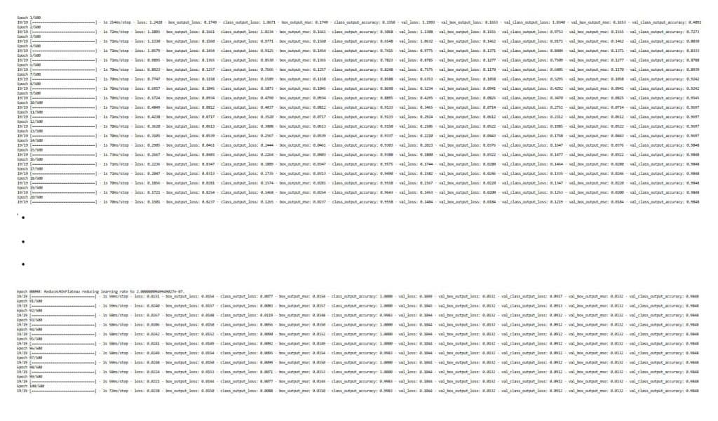
Step 8: Plot Model’s Loss & Accuracy Curves
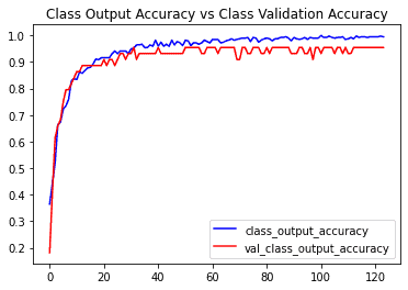
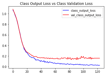
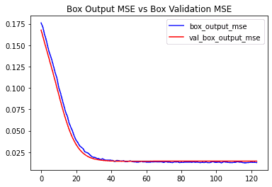
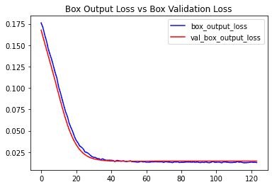
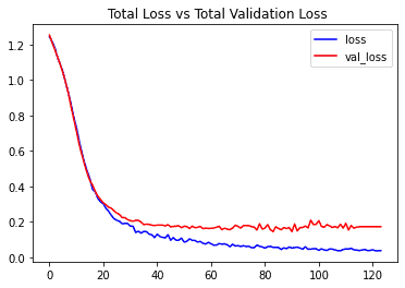
Now we had separate losses and separate metrics for different branches. On top of that we used a validation set. We are now dealing with 10 total metrics. Let’s visualize and understand these by plotting them.
def plot(var1, var2, plot_name):
  # Get the loss metrics from the trained model
  c1 = history.history[var1]
  c2 = history.history[var2]

  epochs = range(len(c1))

  # Plot the metrics
  plt.plot(epochs, c1, 'b', label=var1)
  plt.plot(epochs, c2, 'r', label=var2)
  plt.title(str(plot_name))
  plt.legend()
plot( 'class_output_accuracy', 'val_class_output_accuracy', 'Class Output Accuracy vs Class Validation Accuracy')
plot( 'class_output_loss', 'val_class_output_loss', 'Class Output Loss vs Class Validation Loss')
plot( 'box_output_mse', 'val_box_output_mse', 'Box Output MSE vs Box Validation MSE')
plot('box_output_loss', 'val_box_output_loss', 'Box Output Loss vs Box Validation Loss')
# This is the most important metric, you can take just take a look at this
plot('loss','val_loss', ' Total Loss vs Total Validation Loss')
Code to save your model
# Save your model here in .h5 format.
model.save('caltech.h5')

# Load the saved model
# model = load_model('caltech.h5')
Step 9: Test your model on new images
In this step, we will create a function that will use the model to predict new images.
# Enter your class names in this list
global label_names

# Must be same as the Annotations list we used
label_names = sorted(classes_list)
Predict Function
Here we will create a function that will use the model for prediction with new images input.
# We will use this function to make prediction on images.
def predict(image, returnimage = False,  scale = 0.9):

  # Before we can make a prediction we need to preprocess the image.
  processed_image = preprocess(image)

  # Now we can use our model for prediction
  results = model.predict(processed_image)

  # Now we need to postprocess these results.
  # After postprocessing, we can easily use our results
  label, (x1, y1, x2, y2), confidence = postprocess(image, results)

  # Now annotate the image
  cv2.rectangle(image, (x1, y1), (x2, y2), (0, 255, 100), 2)
  cv2.putText(
      image,
      '{}'.format(label, confidence),
      (x1, y2 + int(35 * scale)),
      cv2.FONT_HERSHEY_COMPLEX, scale,
      (200, 55, 100),
      2
      )

  # Show the Image with matplotlib
  plt.figure(figsize=(10,10))
  plt.imshow(image[:,:,::-1])
Preprocessing Funciton
This function will preprocess new images the same way we did initially, before training.
# This function will preprocess images.
def preprocess(img, image_size = 300):

    image = cv2.resize(img, (image_size, image_size))
    image = cv2.cvtColor(image, cv2.COLOR_BGR2RGB)
    image = image.astype("float") / 255.0

    # Expand dimensions as predict expect image in batches
    image = np.expand_dims(image, axis=0)
    return image
Post Processing Function
After the prediction, you need postprocessing to extract the class label and the real bounding box coordinates.
def postprocess(image, results):

    # Split the results into class probabilities and box coordinates
    bounding_box, class_probs = results

    # First let's get the class label

    # The index of class with the highest confidence is our target class
    class_index = np.argmax(class_probs)

    # Use this index to get the class name.
    class_label = label_names[class_index]

    # Now you can extract the bounding box too.

    # Get the height and width of the actual image
    h, w = image.shape[:2]

    # Extract the Coordinates
    x1, y1, x2, y2 = bounding_box[0]

    # Convert the coordinates from relative (i.e. 0-1) to actual values
    x1 = int(w * x1)
    x2 = int(w * x2)
    y1 = int(h * y1)
    y2 = int(h * y2)

    # return the lable and coordinates
    return class_label, (x1,y1,x2,y2),class_probs
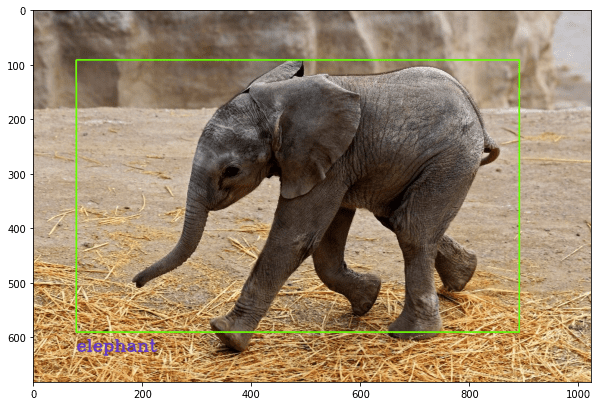
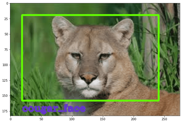
Now that we have created all the required functions, let’s test our model on new images.
!wget -q -O  elephant.jpg https://scx2.b-cdn.net/gfx/news/2020/zoomthebabye.jpg
image = cv2.imread('/content/elephant.jpg' )
predict(image, scale = 1)
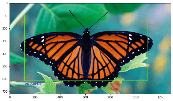
!wget -q -O  butterfly.jpg https://www.sciencemag.org/butterfly.jpg
image = cv2.imread('/content/butterfly.jpg' )
predict(image)
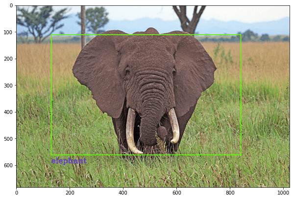
!wget -q -O  elephant2.jpg https://elephants.com/elephant.jpg
image = cv2.imread('/content/elephant2.jpg' )
predict(image)
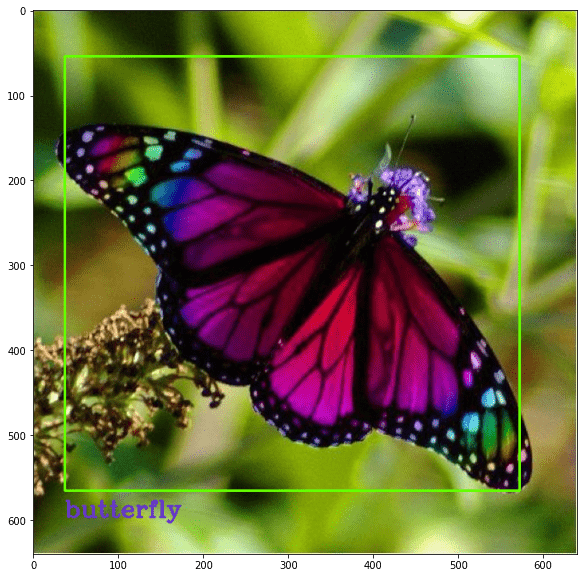
!wget -q -O  butterfly2.jpg https://i.pinimg.com/butterfly.jpg
image = cv2.imread('/content/butterfly2.jpg' )
predict(image)
!wget -q -O  cougar2.jpg https://encrypted-tbn0.gstatic.com/image.jpg
image = cv2.imread('/content/cougar2.jpg' )
predict(image, scale = 0.5)
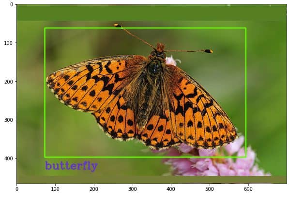
!wget -q -O  butterfly3.jpg https://www.naturepl.com/cache/pcache2/00525060.jpg
image = cv2.imread('/content/butterfly3.jpg' )
predict(image)
Summary & Conclusion:
In this tutorial we learned
- there is another problem that lies between image classification and object detection called Classification with Localization.
- how to perform different kinds of augmentations.
- how to create a multi-output model to output two totally different features.
- how to convert any image classifier to a detector just by adding an extra head.
- how to work with multiple losses and metrics and evaluate them by creating plots.
Here are some drawbacks of the discussed approach.
- The approach is limited by the fact that there should only be one object present per image.
- For the bounding box, we are monitoring Mean squared error which helps but is not the most useful loss to monitor. Ideally, we need to measure the Intersection over Union (IOU) score.
- This setup is, at best is a hack for localization. I would strongly recommend training a SoTA Object Detector using TFOD API for serious localization problems. This gives comparatively better performance with proper Object Detection models.
If you enjoyed this tutorial then be sure to drop a comment.
We would love to hear from you. Ask any questions you want, we would be happy to help!




100K+ Learners
Join Free OpenCV Bootcamp3 Hours of Learning