Deep learning has been one of the fastest-growing technologies in the modern world. Deep learning has become part of our everyday life, from voice-assistant to self-driving cars, it is everywhere. One such application is Automatic License Plate Recognition (ALPR). As the name suggests, ALPR is a technology that uses the power of AI and deep learning to automatically detect and recognize the characters of a vehicle’s license plate. This blog post will focus on the same.
This blog post will focus on end to end implementation of ALPR with a 2 step process, i) License plate detection, ii) OCR of detected license plates.
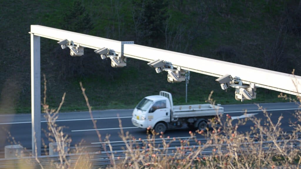
Image credit – Cameramann, CC BY-SA 4.0, via Wikimedia Commons
- Introduction to ALPR
- Working of ALPR
- Detection of license plate using YOLOv4
- OCR
- Inference
- Integration of tracker
- Conclusion
- References
1. Introduction to Automatic License Plate Recognition ALPR
Imagine one beautiful summer you are driving on a highway, your favourite song playing on the radio and you go over the speed limit and drive past a few cameras at a speed of 90Km/h in a 70Km/h speed limit zone and realize your mistake but its too late. A few weeks later you receive a ticket, with evidence as to the image of your car. You must wonder, do they manually check every image and send the tickets?
Not at all, that’s when ALPR comes. From the captured image or footage, ALPR detects and extracts your license plate number and send you the ticket. All of this is because of the simple ALPR system and a few lines of code.
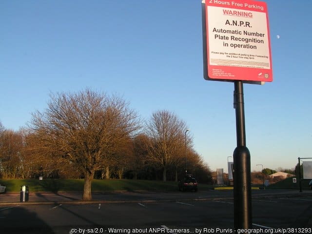
Automatic License Plate Recognition (ALPR) or ANPR is the technology responsible for reading the License plates of a vehicle in an image or a video sequence using optical character recognition. With the latest advancement in Deep Learning and Computer Vision, these tasks can be done in a matter of milliseconds.
Uses
ALPR is a very advanced and intelligent system that has gotten popular due to its various real-life use cases, without any human intervention, Let’s have a look at them.
- Traffic violation: The ALPR can be used by police or law enforcement to identify any traffic violation by a vehicle at a traffic light using only a single camera. It can also be used to identify any stolen or non-registered vehicles in real-time.
- Parking management: Parking management at many places requires a lot of human interaction, But due to ALPR it can be reduced to zero. The camera installed in the parking lots can recognize the plates at the entrance and store them in a database or allow the vehicles only if they are in the database. At the time of exit, the plate can be recognized again and can be charged accordingly.
- Tollbooth payments: At highways, manual toll booths get hectic and can lead to huge traffic. Using ANPR, toll booths can recognize the license plates and receive payments automatically.
But how does ANPR work? Let’s have a look at it in the next section.
2. Working of ALPR
ALPR is one of the widely used computer vision applications. It makes use of various methods like object detection, OCR, segmentation, etc. For hardware, the ALPR system only requires a camera and a good GPU. To make it simple this blog post will focus on a two-step process.
- Detection: Firstly, an image or a frame of the video sequence is passed to the detection algorithm from a camera or an already stored file, which detects the license plate and returns the bounding box location of that plate.
- Recognition: The OCR is applied to the detected license plate for recognizing the characters of the plate and returns the characters in the same order in text format. The output can be stored in a database or can be plotted on the image for visualization.
Let’s look at each step in detail one by one in Google Colaboratory.
3. Detection of License plate using YOLOv4
This module of the pipeline is responsible for detecting the number plate from the image or frame of the video sequence.
The detection process can be done using any detector whether it’s a region-based detector or a single shot detector. This blog post will focus on one such single shot detector known as YOLOv4, mainly because of its good speed and accuracy tradeoff and ability to detect small objects better. YOLOv4 will be implemented using the darknet framework.
Darknet

Darknet is an open-source neural network framework written in C and CUDA. YOLOv4 uses CSPDarknet53 CNN which means, its backbone for object detection uses Darknet53 which has a total of 53 convolutional layers. Darknet is very easy to install, use, and can be done in just a few lines of code.
!git clone https://github.com/AlexeyAB/darknet
Darknet will be installed and compiled and some parameters will be set according to the environment needs.
%cd darknet
!sed -i 's/OPENCV=0/OPENCV=1/' Makefile
!sed -i 's/GPU=0/GPU=1/' Makefile
!sed -i 's/CUDNN=0/CUDNN=1/' Makefile
!sed -i 's/CUDNN_HALF=0/CUDNN_HALF=1/' Makefile
!sed -i 's/LIBSO=0/LIBSO=1/' Makefile

!make
Congrats! Darknet is now installed.
Here, some parameters like OpenCV, GPU, CUDA etc. are set to 1 that is set as True, as they will be needed to make the code efficient and run computations faster.
Dataset
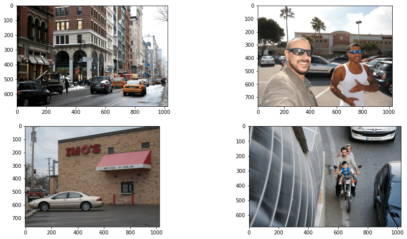
Data is the core of any AI application and one of the first and most important steps. For training the YOLOv4 detector Google open images dataset of vehicles will be used. Google’s “Open Images” is an open-source dataset with thousands of images of objects with annotations for object detection, segmentation etc.
This dataset consists of 1500 training images and 300 validation images in the YOLO format. Dataset can be downloaded from here and put under the folder /darknet/data. Let’s have a look at the dataset.
import math
# Creating a list of image files of the dataset.
data_path = './data/obj/train/'
files = os.listdir(data_path)
img_arr = []

# Displaying 4 images only.
num = 4

# Appending the array of images to a list.
for fimg in files:
    if fimg.endswith('.jpg'):
      demo = img.imread(data_path+fimg)
      img_arr.append(demo)
      if len(img_arr) == num:
        break

# Plotting the images using matplotlib.
_, axs = plt.subplots(math.floor(num/2), math.ceil(num/2), figsize=(50, 28))

axs = axs.flatten()

for cent, ax in zip(img_arr, axs):
    ax.imshow(cent)
plt.show()
Training
To make the model learn, it needs to be trained on the dataset. Before starting the training process, the config file(.cfg) needs to be modified. The parameters that need modifications are batch size, subdivision, classes, etc. Download the config file from here and put it under the /darknet/cfg folder.
Now the data is already in place, the configuration is done, but how will the model access the data? Two files are created, one of which contains the information of train data, test data, and information about classes. Let’s call it obj.data (can be downloaded from here) and the other is obj.names which contains the names of all the classes. You can download obj.names from here.
# Creating a folder checkpoint to save weights while training.
%cd ../
!mkdir checkpoint
The next step is to download the pre-trained weights of YOLOv4.
!wget https://github.com/AlexeyAB/darknet/releases/download/darknet_yolo_v3_optimal/yolov4.conv.137
Now comes the important part that is TRAINING!
!./darknet detector train data/obj.data cfg/yolov4-obj.cfg yolov4.conv.137 -dont_show -map
The arguments include obj.data file, config file, and yolov4 pre-trained weights as discussed earlier.
-dont_showis passed when we don’t want to display the output. Also, this needs to be passed when running the code in google colab notebook as it does not support GUI output and will result in an error when not passed.
-mapis passed to calculate mAP of the predictions after every few iterations.
Let’s wait for a few hours and HURRAY! The model is now trained. If you want to skip the training process, the trained or our fine-tuned model can also be downloaded from here. Also, Access the Notebook here.
Evaluation
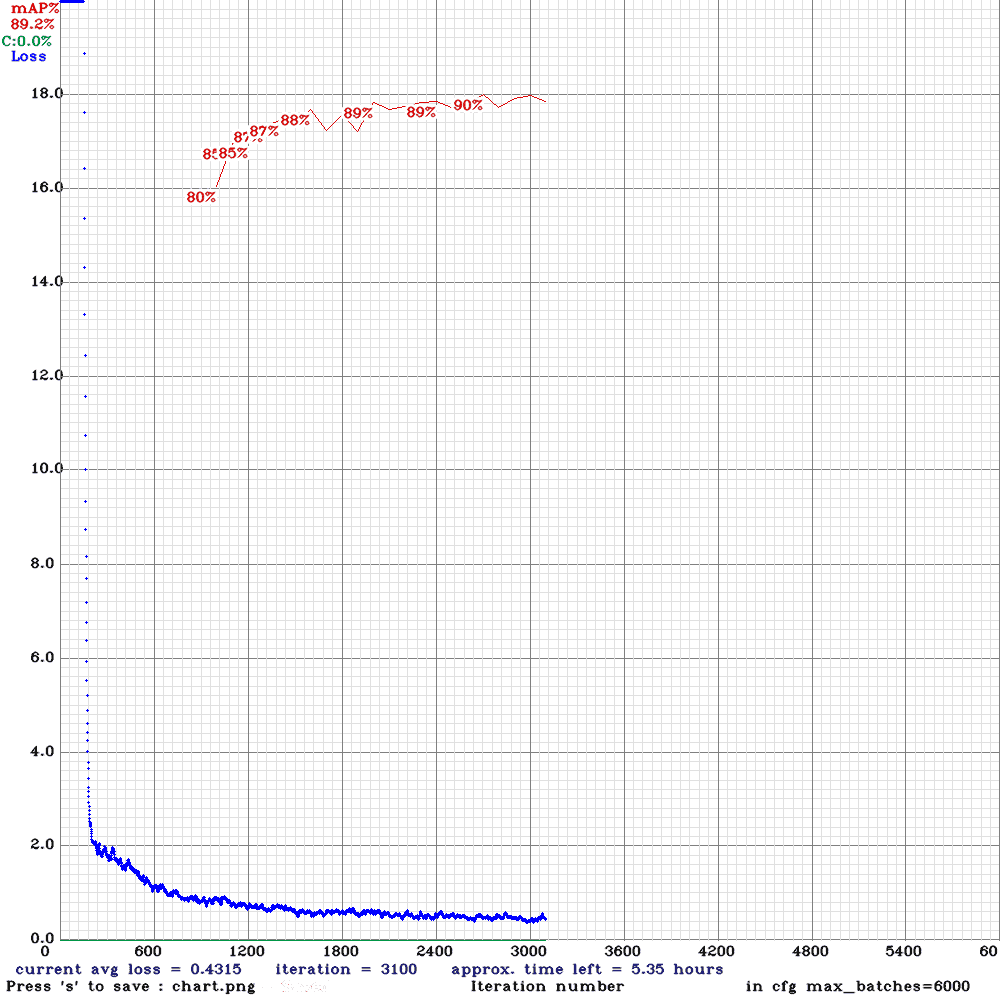
It is very important to judge the trained model’s performance on unseen data. It is a good way to know whether the model is performing well or overfitting. For object detection tasks, one such metric is mean average precision in short known as mAP. On a high-level explanation, the predicted bounding box is compared with the detected bounding box and a score is returned which is called mAP.
This code automatically saves the training progress chart, here’s how our model performed, achieving 90% mAP after 3000 epochs in 5.3 hours.
Inference
Now the license plate detector is fully trained. It is time to put it to use. For this, we will create a helper function called yolo_det(). This function is responsible for detecting the bounding boxes of the license plates from the input vehicle images.
def yolo_det(frame, config_file, data_file, batch_size, weights, threshold, output, network, class_names, class_colors, save = False, out_path = ''):

  prev_time = time.time()

  # Preprocessing the input image.
  width = darknet.network_width(network)
  height = darknet.network_height(network)
  darknet_image = darknet.make_image(width, height, 3)
  image_rgb = cv2.cvtColor(frame, cv2.COLOR_BGR2RGB)
  image_resized = cv2.resize(image_rgb, (width, height))

  # Passing the image to the detector and store the detections
  darknet.copy_image_from_bytes(darknet_image, image_resized.tobytes())
  detections = darknet.detect_image(network, class_names, darknet_image, thresh=threshold)
  darknet.free_image(darknet_image)

  # Plotting the deetections using darknet in-built functions
  image = darknet.draw_boxes(detections, image_resized, class_colors)
  print(detections)
  if save:
    im = cv2.cvtColor(image, cv2.COLOR_RGB2BGR)
    file_name = out_path + '-det.jpg'
    cv2.imwrite(os.path.join(output, file_name), im)

  # Calculating time taken and FPS for detection
  det_time = time.time() - prev_time
  fps = int(1/(time.time() - prev_time))
  print("Detection time: {}".format(det_time))

  # Resizing predicted bounding box from 416x416 to input image resolution
  out_size = frame.shape[:2]
  in_size = image_resized.shape[:2]
  coord, scores = resize_bbox(detections, out_size, in_size)
  return coord, scores, det_time
Let’s define a function resize_bbox() for resizing the predicted bounding box coordinates back to bounding box coordinates according to the original image size. When the image is passed through the detector, the image should be resized to a certain resolution. The detector also outputs the result with the same resolution, in this case, 416×416. To convert the image back to its input resolution, it is needed to change the bounding box coordinates accordingly.
def resize_bbox(detections, out_size, in_size):
  coord = []
  scores = []

  # Scaling the bounding boxes according to the original image resolution.
  for det in detections:
    points = list(det[2])
    conf = det[1]

    xmin, ymin, xmax, ymax = darknet.bbox2points(points)
    y_scale = float(out_size[0]) / in_size[0]
    x_scale = float(out_size[1]) / in_size[1]
    ymin = int(y_scale * ymin)
    ymax = int(y_scale * ymax)
    xmin = int(x_scale * xmin) if int(x_scale * xmin) > 0 else 0
    xmax = int(x_scale * xmax)

    final_points = [xmin, ymin, xmax-xmin, ymax-ymin]
    scores.append(conf)
    coord.append(final_points)

  return coord, scores
4. OCR
Now that we have trained the custom license plate detector, It’s time to move on to the second step of the ALPR which is Text Recognition.
Text recognition is the process of recognizing text from a scenario by understanding and analyzing its underlying patterns. It is also known as optical character recognition or OCR. It can also be used in various applications like document reading, information retrieval, product identification from shelves, and many more. OCR can either be trained or used as a pre-trained model. In this article, a pre-trained model of OCR will be used.
PaddleOCR
One such framework or toolkit for OCR is PaddleOCR. PaddleOCR offers users multilingual practical OCR tools that help the users to apply and train different models in a few lines of code. PaddleOCR offers a lot of models in its toolkit, including PP-OCR, a series of high-quality pre-trained OCR, the latest algorithms such as SRN, and popular OCR algorithms like CRNN.
PaddleOCR also provides different kinds of models whether it’s lightweight (a model which takes less memory) or heavyweight(a model which takes large memory) along with its pre-trained weights to use freely.
OCR Comparison
As explained in the previous section that PaddleOCR provides various models, It is always a good practice to compare which model performs well in case of accuracy as well as speed.
The models were tested on the IC15 dataset which is an incidental scene text dataset, containing only English words. It contains 1000 training images, but it was tested on a random of 500 images from it. The model is tested using a string similarity metric known as Levenshtein distance. Levenshtein distance is the changes required in a string to achieve another string. The less the distance the better the model will be. Three models are tested on the IC15 dataset using Levenshtein distance on the Tesla K80 GPU.

Table: 01-ocr-comparison
The focus will be on the lightweight PPOCRv2(11.6M). It has a good trade-off between speed, accuracy and is also very lightweight (i.e taking very less memory). It also offers support for both English and Chinese languages. For the OCR comparison code refer here.
OCR implementation
Now, it is time to implement the selected OCR model. PaddleOCR will be implemented in a few lines of code and will perform wonders for our ALPR system.
First off, let’s install the required toolkits and dependencies. These dependencies and tools will help us access all the required files and scripts needed for OCR implementation.
# Navigating to previous directory or home directory
%cd ../
# Installing dependencies
!pip install paddlepaddle-gpu
!pip install "paddleocr>=2.0.1"
After the installation, The OCR needs to be initialized according to our requirements.
from paddleocr import PaddleOCR
ocr = PaddleOCR(lang='en',rec_algorithm='CRNN')
Using PaddleOCR we initialize our OCR, it takes several arguments, which are:
lang– specifies the language to be recognizeddet_algorithm– specifies the text detection algorithm usedRec_algorithm– specifies the recognition algorithm used
For ALPR, only two arguments will be passed, that is of language and recognition algorithm. Here we have used lang as english and CRNN recognition algorithm which is also called PPOCRv2 in this toolkit.
This OCR can be used using just one line of code.
# Syntax
result = ocr.ocr(cr_img, cls=False, det=False)
Here, cr_img is the image passed to OCR, cls , and det are the arguments that are set as false because there is no need for a text detector and text angle classifier in our ALPR pipeline.
5. Inference
Now that the license plate detector is fully trained, OCR is up and ready. It is time to put all of these together and put them to use. For this, we will be going to create some helper functions to access all of the functionalities in one go.
First of all, we will create a function that will be responsible for cropping the image by taking the image and coordinates as parameters, Let’s call it crop().
def crop(image, coord):
  # Cropping is done by -> image[y1:y2, x1:x2].
  cr_img = image[coord[1]:coord[3], coord[0]:coord[2]]
  return cr_img
Testing on images
For performing ANPR on images, we will create a final function, say test_img() which will be performing detection, cropping, OCR and plotting of output in one place.
Before that, we will initialize some variables that will be helpful throughout the whole blog post.
# Variables storing colors and fonts.
font = cv2.FONT_HERSHEY_SIMPLEX
blue_color = (255,0,0)
white_color = (255,255,255)
black_color = (0,0,0)
green_color = (0,255,0)
yellow_color = (178, 247, 218)
def test_img(input, config_file, weights, out_path):
  # Loading darknet network and classes along with the bbox colors.
  network, class_names, class_colors = darknet.load_network(
            config_file,
            data_file,
            weights,
            batch_size= batch_size
        )

  # Reading the image and performing YOLOv4 detection.
  img = cv2.imread(input)
  bboxes, scores, det_time = yolo_det(img, config_file, data_file, batch_size, weights, thresh, out_path, network, class_names, class_colors)

  # Extracting or cropping the license plate and applying the OCR.
  for bbox in bboxes:
 bbox = [bbox[0], bbox[1], bbox[2]- bbox[0], bbox[3] - bbox[1]]
    cr_img = crop(img, bbox)
    result = ocr.ocr(cr_img, cls=False, det=False)
    ocr_res = result[0][0]
    rec_conf = result[0][1]

    # Plotting the predictions using OpenCV.
    (label_width,label_height), baseline = cv2.getTextSize(ocr_res , font, 2, 3)
    top_left = tuple(map(int,[int(bbox[0]),int(bbox[1])-(label_height+baseline)]))
    top_right = tuple(map(int,[int(bbox[0])+label_width,int(bbox[1])]))
    org = tuple(map(int,[int(bbox[0]),int(bbox[1])-baseline]))

    cv2.rectangle(img, (int(bbox[0]), int(bbox[1])), (int(bbox[2]), int(bbox[3])), blue_color, 2)
    cv2.rectangle(img, top_left, top_right, blue_color,-1)
    cv2.putText(img, ocr_res, org, font, 2, white_color,3)

  # Writing output image.
  file_name = os.path.join(out_path, 'out_' + input.split('/')[-1])
  cv2.imwrite(file_name, img)
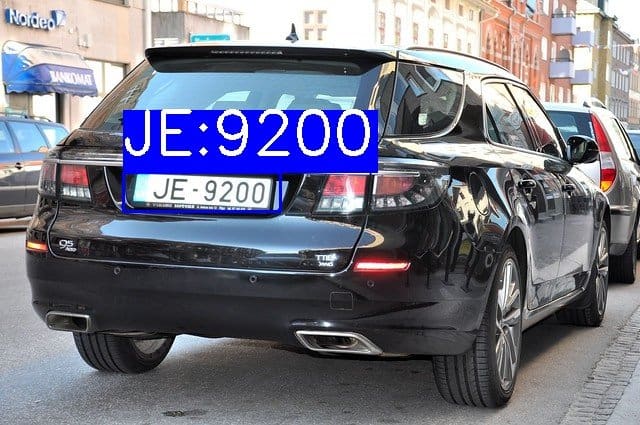
Congrats!! The pipeline for running ALPR on an image is successfully created. Let’s try it on a random image.

First, we will import some libraries and required functionalities and methods to apply ANPR.
# Importing libraries and required functionalities.
# Required libraries.
import os
import glob
import random
import time
import cv2
import numpy as np
import subprocess
import sys
from PIL import Image
import matplotlib
import matplotlib.pyplot as plt
%matplotlib inline

# Darknet object detector imports.
%cd ./darknet
import darknet
from darknet_images import load_images
from darknet_images import image_detection
%cd ../
# Add absolute paths according to your folder structure.
# Declaring important variables.
# Path of Configuration file of YOLOv4.
config_file = '/content/gdrive/MyDrive/yolov4-darknet/darknet/cfg/yolov4-obj.cfg'
# Path of obj.data file.
data_file = '/content/gdrive/MyDrive/yolov4-darknet/darknet/data/obj.data'
# Batch size of data passed to the detector.
batch_size = 1
# Path to trained YOLOv4 weights.
weights = '/content/gdrive/MyDrive/yolov4-darknet/checkpoint/yolov4-obj_best.weights'
# Confidence threshold.
thresh = 0.6
# Calling the function.
input_dir = 'car-img.jpg'
out_path = '/content/'
test_img(input_dir, config_file, weights,out_path)
We will display the final output now.
out_img = cv2.imread('./out_car-img.jpg')
cv2.imshow(out_img)
Testing on videos
After we have tested our ALPR on image, we can similarly apply this to the video as well. For video, we just apply the ALPR pipeline frame by frame in the similar manner as the image. Let’s dive right into it.
def test_vid(vid_dir, config_file, weights,out_path):
  # Declaring variables for video processing.
  cap = cv2.VideoCapture(vid_dir)
  codec = cv2.VideoWriter_fourcc(*'XVID')
  width = int(cap.get(cv2.CAP_PROP_FRAME_WIDTH))
  height = int(cap.get(cv2.CAP_PROP_FRAME_HEIGHT))
  fps = int(cap.get(cv2.CAP_PROP_FPS))
  file_name = os.path.join(out_path, 'out_' + vid_dir.split('/')[-1])
  out = cv2.VideoWriter(file_name, codec, fps, (width, height))

  # Frame count variable.
  ct = 0

  # Loading darknet network and classes along with the bbox colors.
  network, class_names, class_colors = darknet.load_network(
          config_file,
          data_file,
          weights,
          batch_size= batch_size
      )

  # Reading video frame by frame.
  while(cap.isOpened()):
    ret, img = cap.read()
    if ret == True:
        print(ct)

        # Noting time for calculating FPS.
        prev_time = time.time()

        # Performing the YOLOv4 detection.
        bboxes, scores, det_time = yolo_det(img, config_file, data_file, batch_size, weights, thresh, out_path, network, class_names, class_colors)

        # Extracting or cropping the license plate and applying the OCR.
        if list(bboxes):
          for bbox in bboxes:
            bbox = [bbox[0], bbox[1], bbox[2]- bbox[0], bbox[3] - bbox[1]]
            cr_img, cord = crop(img, bbox)

            result = ocr.ocr(cr_img, cls=False, det=False)

            ocr_res = result[0][0]
            rec_conf = result[0][1]

            # Plotting the predictions using OpenCV.
            txt = ocr_res
            (label_width,label_height), baseline = cv2.getTextSize(ocr_res , font,2,3)
            top_left = tuple(map(int,[int(bbox[0]),int(bbox[1])-(label_height+baseline)]))
            top_right = tuple(map(int,[int(bbox[0])+label_width,int(bbox[1])]))
            org = tuple(map(int,[int(bbox[0]),int(bbox[1])-baseline]))

            cv2.rectangle(img, (int(bbox[0]), int(bbox[1])), (int(bbox[2]), int(bbox[3])), blue_color, 2)
            cv2.rectangle(img, top_left, top_right, blue_color, -1)
            cv2.putText(overlay_img,txt, org, font, 2, white_color, 3)
            #cv2.imwrite('/content/{}.jpg'.format(ct), img)

          # Calculating time taken and FPS for the whole process.
          tot_time = time.time() - prev_time
          fps = 1/tot_time

          # Writing information onto the frame and saving it to be processed in a video.
          cv2.putText(img, 'frame: %d fps: %s' % (ct, fps),
                  (0, int(100 * 1)), cv2.FONT_HERSHEY_PLAIN, 5, (0, 0, 255), thickness=2)
          out.write(img)

        ct = ct + 1
    else:
      break
Time to try it on a random video. You can download it from here.
# Calling the function.
input_dir = './Pexels Videos 2103099.mp4'
out_path = '/content/'
test_vid(input_dir, config_file, weights,out_path)
Displaying the output (for jupyter notebooks or colab).
from IPython.display import HTML
from base64 import b64encode

# Input video path.
save_path = './out_Pexels Videos 2103099.mp4'

# Compressed video path.
compressed_path = "./compressed.mp4"

#compressing the size of video to avoid crashing.
os.system(f"ffmpeg -i {save_path} -vcodec libx264 {compressed_path}")

# Show video.
mp4 = open(compressed_path,'rb').read()
data_url = "data:video/mp4;base64," + b64encode(mp4).decode()
HTML("""
<video width=400 controls>
      <source src="%s" type="video/mp4">
</video>
""" % data_url)
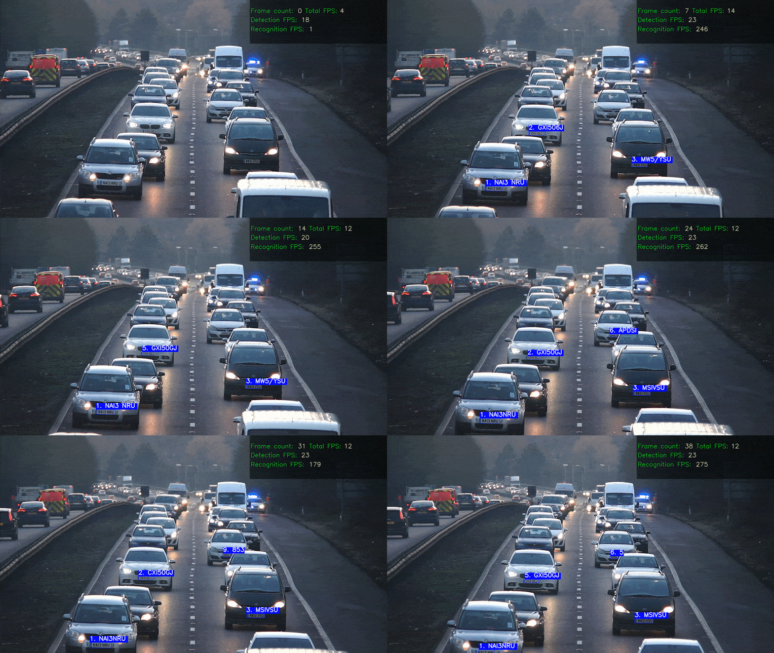
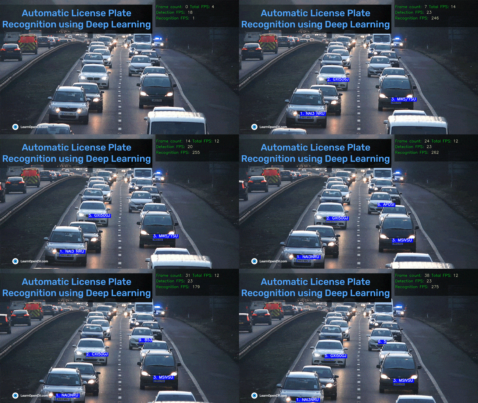
Output can be seen here.
6. Integration of Tracker
As you must have seen in the previous section, The video outputs are not much accurate there are many issues with it.
- Jittering
- Fluctuation of OCR output
- Loss of detection
To deal with this problem, This section proposes a solution that is integrating a tracker with the ALPR system. But how does the use of a tracker solve these problems? Let’s have a look at it.
Role of Tracker in ALPR
When running ALPR on a video, it causes some issues which makes the ALPR less accurate, as discussed earlier. But if the tracker is used, these issues can be rectified. Tracker is generally used for the following reasons:
- Working when object detection fails
- Assigning ids
- Tracking paths
All of the problems the ALPR is facing, tracker is only used because of these problems. The tracker will be used for getting the best OCR result of a particular detected license plate.
After the tracker is implemented, it returns the coordinates of the bounding box and ids along with it OCR will be applied to every bounding box and the output will be stored along with id. To reduce the problem of fluctuation of OCR output, all the bounding boxes of the same ids will be collected till the current frame and the bounding box with the highest OCR confidence will be kept and displayed for that id. The process will be more clear when implemented.
Implementation of Tracker
Firstly, We will clone the original DeepSORT repository.
# Cloning DeepSORT
!git clone https://github.com/nwojke/deep_sort.git
Before we further move on, The original DeepSORT repo uses a deprecated sklearn function called linear_assignment, which needs to be replaced for smooth and error-free execution of code. To replace this, we will be using scipy library.
For this first open the file /deep_sort/deep_sort/linear_assignment.py.
- Replace from sklearn.utils.linear_assignment_ import linear_assignment in line 4 with from scipy.optimize import linear_sum_assignment.
- After the correct import, We will now put it to use.
Replace indices = linear_assignment(cost_matrix) in line 58 with the following lines of code:
indices = linear_sum_assignment(cost_matrix)
indices = np.asarray(indices)
indices = np.transpose(indices)
Also, rename /deep_sort/tools folder as /deep_sort/tools_deepsort to avoid any name overlapping.
After we have successfully installed and cloned the DeepSORT code, Let’s create a new helper function get_best_ocr(), to implement the logic discussed in the previous section.
def get_best_ocr(preds, rec_conf, ocr_res, track_id):
  for info in preds:
    # Check if it is the current track id.
    if info['track_id'] == track_id:
      # Check if the ocr confidence is highest or not.
      if info['ocr_conf'] < rec_conf:
        info['ocr_conf'] = rec_conf
        info['ocr_txt'] = ocr_res
      else:
        rec_conf = info['ocr_conf']
        ocr_res = info['ocr_txt']
      break
  return preds, rec_conf, ocr_res
Finally, we will work on the next function of running Automatic License Plate Recognitionon video along with tracker called tracker_test_vid(). It will be just like test_vid(), but with a tracker implemented with it. This blog post will focus on using DeepSORT as the tracker, because it’s lightweight easy to use and also provides an appearance descriptor and that too in just a few lines of code. We will be using the pretrained deep association metric model called mars-small128.pb, which can be downloaded from here.
def tracker_test_vid(vid_dir, config_file, weights,out_path):
  # Declaring variables for video processing.
  cap = cv2.VideoCapture(vid_dir)
  codec = cv2.VideoWriter_fourcc(*'XVID')
  width = int(cap.get(cv2.CAP_PROP_FRAME_WIDTH))
  height = int(cap.get(cv2.CAP_PROP_FRAME_HEIGHT))
  fps = int(cap.get(cv2.CAP_PROP_FPS))
  file_name = os.path.join(out_path, 'out_' + vid_dir.split('/')[-1])

  out = cv2.VideoWriter(file_name, codec, fps, (width, height))

  # Declaring variables for tracker.
  max_cosine_distance = 0.4
  nn_budget = None

  # Initializing tracker
  model_filename = './model_data/mars-small128.pb'
  encoder = gdet.create_box_encoder(model_filename, batch_size=1)
  metric = nn_matching.NearestNeighborDistanceMetric("cosine", max_cosine_distance, nn_budget)
  tracker = Tracker(metric)

  # Initializing some helper variables.
  ct = 0
  preds = []
  total_obj = 0
  rec_tot_time = 1
  alpha = 0.5

  # Loading darknet network and classes along with the bbox colors.
  network, class_names, class_colors = darknet.load_network(
          config_file,
          data_file,
          weights,
          batch_size= batch_size
      )

  # Reading video frame by frame.
  while(cap.isOpened()):
    ret, img = cap.read()
    if ret == True:

        h, w = img.shape[:2]
        print(ct)

        w_scale = w/1.55
        h_scale = h/17

        # Method to blend two images, here used to make the information box transparent.
        overlay_img = img.copy()
        cv2.rectangle(img, (int(w_scale), 0), (w, int(h_scale*3.4)), (0,0,0), -1)
        cv2.addWeighted(img, alpha, overlay_img, 1 - alpha, 0, overlay_img)

        # Noting time for calculating FPS.
        prev_time = time.time()

        # Performing the YOLOv4 detection.
        bboxes, scores, det_time = yolo_det(img, config_file, data_file, batch_size, weights, thresh, out_path, network, class_names, class_colors)

        if list(bboxes):
          # Getting appearance features of the object.
          features = encoder(img, bboxes)
          # Storing all the required info in a list.
          detections = [Detection(bbox, score, feature) for bbox, score, feature in zip(bboxes, scores, features)]

          # Applying tracker.
          # The tracker code flow: kalman filter -> target association(using hungarian algorithm) and appearance descriptor.
          tracker.predict()
          tracker.update(detections)
          track_time = time.time() - prev_time

          # Checking if tracks exist.
          for track in tracker.tracks:
            if not track.is_confirmed() or track.time_since_update > 1:
                continue

            # Changing track bbox to top left, bottom right coordinates
            bbox = list(track.to_tlbr())

            for i in range(len(bbox)):
              if bbox[i] < 0:
                bbox[i] = 0

            # Extracting or cropping the license plate and applying the OCR.
            cr_img = crop(img, bbox)

            rec_pre_time = time.time()
            result = ocr.ocr(cr_img, cls=False, det=False)
            rec_tot_time = time.time() - rec_pre_time

            ocr_res = result[0][0]
            print(result)
            rec_conf = result[0][1]

            if rec_conf == 'nan':
              rec_conf = 0

            # Storing the ocr output for corresponding track id.
            output_frame = {"track_id":track.track_id, "ocr_txt":ocr_res, "ocr_conf":rec_conf}

            # Appending track_id to list only if it does not exist in the list.
            if track.track_id not in list(set(ele['track_id'] for ele in preds)):
              total_obj = total_obj + 1
              preds.append(output_frame)
            # Looking for the current track in the list and updating the highest confidence of it.
            else:
              preds, rec_conf, ocr_res = get_best_ocr(preds, rec_conf, ocr_res, track.track_id)

            # Plotting the predictions using OpenCV.
            txt = str(track.track_id) + '. ' + ocr_res
            (label_width,label_height), baseline = cv2.getTextSize(txt , font,2,3)
            top_left = tuple(map(int,[int(bbox[0]),int(bbox[1])-(label_height+baseline)]))
            top_right = tuple(map(int,[int(bbox[0])+label_width,int(bbox[1])]))
            org = tuple(map(int,[int(bbox[0]),int(bbox[1])-baseline]))

            cv2.rectangle(overlay_img, (int(bbox[0]), int(bbox[1])), (int(bbox[2]), int(bbox[3])), blue_color, 2)
            cv2.rectangle(overlay_img, top_left, top_right, blue_color, -1)
            cv2.putText(overlay_img,txt, org, font, 2, white_color, 3)
            #cv2.imwrite('/content/{}.jpg'.format(ct), img)

          # Calculating time taken and FPS for the whole process.
          tot_time = time.time() - prev_time
          fps = 1/tot_time

          # Writing information onto the frame and saving the frame to be processed into a video with title and values of different colors.
          if w < 2000:
            size = 1
          else:
            size = 2

          # Plotting frame count information on the frame.
          (label_width,label_height), baseline = cv2.getTextSize('Frame count:' , font,size,2)
          top_left = (int(w_scale) + 10, int(h_scale))
          cv2.putText(overlay_img, 'Frame count:', top_left, font, size, green_color, thickness=2)

          top_left_r1 = (int(w_scale) + 10 + label_width, int(h_scale))
          cv2.putText(overlay_img,'%d ' % (ct), top_left_r1, font, size, yellow_color, thickness=2)

          (label_width,label_height), baseline = cv2.getTextSize('Frame count:' + ' ' + str(ct) , font, size,2)
          top_left_r1 = (int(w_scale) + 10 + label_width, int(h_scale))
          cv2.putText(overlay_img, 'Total FPS:' , top_left_r1, font, size, green_color, thickness=2)

          (label_width,label_height), baseline = cv2.getTextSize('Frame count:' + ' ' + str(ct) + 'Total FPS:' , font, size,2)
          top_left_r1 = (int(w_scale) + 10 + label_width, int(h_scale))
          cv2.putText(overlay_img, '%s' % (int(fps)), top_left_r1, font, size, yellow_color, thickness=2)

          # Plotting Total FPS of ANPR information on the frame.
          cv2.putText(overlay_img, 'Detection FPS:' ,(top_left[0], int(h_scale*1.7)), font, size, green_color, thickness=2)
          (label_width,label_height), baseline = cv2.getTextSize('Detection FPS:', font,size,2)
          cv2.putText(overlay_img, '%d' % ((int(1/det_time))),(top_left[0] + label_width, int(h_scale*1.7)), font, size, yellow_color, thickness=2)

          # Plotting Recognition/OCR FPS of ANPR on the frame.
          cv2.putText(overlay_img, 'Recognition FPS:',(top_left[0], int(h_scale*2.42)), font, size, green_color, thickness=2)
          (label_width,label_height), baseline = cv2.getTextSize('Recognition FPS:', font,size,2)
          cv2.putText(overlay_img, '%s' % ((int(1/rec_tot_time))),(top_left[0] + label_width, int(h_scale*2.42)), font, size, yellow_color, thickness=2)
          cv2.imwrite('/content/{}.jpg'.format(ct), overlay_img)
          out.write(overlay_img)

        # Increasing frame count.
        ct = ct + 1
    else:
      break
Now, We will import the required functions and methods needed to apply DeepSORT. We have already imported other dependencies in earlier sections so no need to import again.
# DeepSORT imports.
%cd ./deep_sort
from application_util import preprocessing
from deep_sort import nn_matching
from deep_sort.detection import Detection
from deep_sort.tracker import Tracker
from tools_deepsort import generate_detections as gdet
import uuid
Run it similarly as previous sections.
# Calling the function.
%cd ../
input_dir = './Pexels Videos 2103099.mp4'
out_path = '/content/'
tracker_test_vid(input_dir, config_file, weights,out_path)
Output can be displayed as shown earlier. Here is the final output, as it is clearly seen that all of the discussed problems are heavily reduced and the ALPR seems pretty accurate and performs with a good speed of 14-15 FPS. The whole inference code can be accessed from this notebook.
7. Conclusion
In this blog post, we built an Automatic License Plate Recognition or ANPR system with a speed of 14 to 15 FPS. Here, We focussed on a two-step process: i) License plate detector, ii) Extraction and OCR of license plate detector.
While going through this, many questions might have hit your brain like, how to speed it up? How to increase accuracy? How will the tracker respond to occlusion? etc. The one way is to try and find out on your own.
Here, the license plate got trained with pretty good accuracy of 90%. If speed is the main goal for license plate detectors, it is more desirable to use YOLO-tiny, which provides better speed than YOLOv4 but with a trade-off with accuracy.
Also, the PaddleOCR’s PP-OCR works flawlessly, it being lightweight as well and pretty accurate which gives a good tradeoff between accuracy and speed. PaddleOCR provides various models like SRN, heavyweight PPOCR and many more, which can be used or even trained from scratch to achieve desirable results.
But the ideal method for our ALPR is to use a tracker with it, which keeps the best OCR result out of all. Various other trackers like OpenCV trackers, CenterTrack, Tracktor etc. which tackle different advanced problems like occlusion, Re-id etc.
Have fun exploring the references, tweaking the inputs, and finding out more ways to make the task more challenging.
8. References
YOLOv4 – https://github.com/AlexeyAB/darknet
License plate Dataset – https://storage.googleapis.com/openimages/web/index.html
PaddleOCR – https://github.com/PaddlePaddle/PaddleOCR
Test video – https://www.pexels.com/video/traffic-flow-in-the-highway-2103099/
DeepSORT – https://github.com/nwojke/deep_sort



100K+ Learners
Join Free OpenCV Bootcamp3 Hours of Learning