Ideas in Machine Learning have a “winner takes all” quality. When an idea takes off, it dominates the field so completely that one tends to believe it is the only idea worth pursuing.
Today, Deep Learning is cool. A few years back learning algorithms like Random Forests and Support Vector Machines (SVMs) were just as cool.
These traditional methods have some benefits over Deep Learning in certain application domains. They sometimes need less data to train on and it takes minutes ( instead of hours or days ) to train. Authors of this paper discovered,
“For example, recently, deep learning was used to find which questions in the Stack Overflow programmer discussion forum can be linked together. That deep learning system took 14 hours to execute. We show here that applying a very simple optimizer called DE to fine tune SVM, it can achieve similar (and sometimes better) results. The DE approach terminated in 10 minutes; i.e. 84 times faster hours than deep learning method.”
Faster training time means you can perform more experiments and bring a product to market faster. A good machine learning engineer is not married to a specific technique. They learn a bag of tools and apply the right tool for the right problem.
In this post, we will learn a math-free intuition behind linear and non-linear Support Vector Machines (SVMs).
What are Support Vector Machines (SVMs)?
The easiest way to understand SVM is using a binary classification problem.
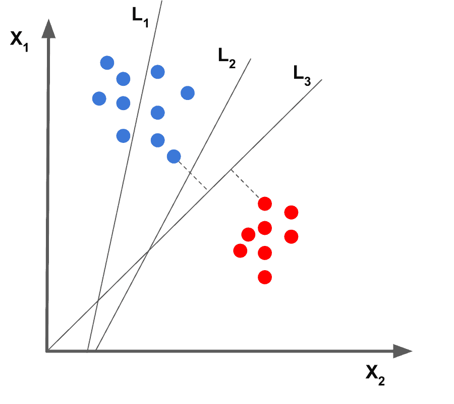
In Figure 1, we see data represented as dots on a 2D plane. The data belongs to two different classes indicated by the color of the dots. One way to learn to distinguish between the two classes is to draw a line that partitions the 2D space into two parts. Training the system simply means finding the line. Once you have trained the system (i.e. found the line), you can say if a new data point belongs to the blue or the red class by simply checking on which side of the line it lies.
In Figure 1, it is clear that line L1 is not a good choice because it does not separate the two classes. L2 and L3 both separate the two classes, but intuitively we know L3 is a better choice than L2 because it more cleanly separates the two classes.
How do Support Vector Machines (SVMs) work?
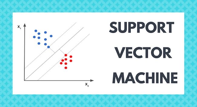
Support Vector Machine (SVM) essentially finds the best line that separates the data in 2D. This line is called the Decision Boundary.
If we had 1D data, we would separate the data using a single threshold value. If we had 3D data, the output of SVM is a plane that separates the two classes. Finally, if the data is more than three dimensions, the decision boundary is a hyperplane which is nothing but a plane in higher dimensions. No, you cannot visualize it, but you get the idea!
Now, let’s see how is line L3 chosen by the SVM.

The points closest to the separating hyperplanes are called the Support Vectors. SVM solves an optimization problem such that
- Support Vectors have the greatest possible distance from the decision boundary (i.e. separating hyperplane).
- The two classes lie on different sides of the hyperplane.
This optimization problem is equivalent to maximizing the Geometric Margin (![]() ) shown in the equation below.
) shown in the equation below.
(1) 
where ![]() is a training example,
is a training example, ![]() takes two values ( 1 and -1 ) for a binary classifier and the separating hyperplane is parameterized by
takes two values ( 1 and -1 ) for a binary classifier and the separating hyperplane is parameterized by ![]() and
and ![]() . In our 2D example,
. In our 2D example, ![]() is simply the coordinates of the 2D points,
is simply the coordinates of the 2D points, ![]() is the 1 for blue and -1 for red dots, and the parameters
is the 1 for blue and -1 for red dots, and the parameters ![]() and
and ![]() are related to the slope and intercept of the separating line.
are related to the slope and intercept of the separating line.
SVM Parameter C
Now, you may be thinking the toy example I picked was too easy and real data is noisy and almost never so neatly separable using a hyperplane.
In such cases, SVM still finds the best hyperplane by solving an optimization problem that tries to increase the distance of the hyperplane from the two classes while trying to make sure many training examples are classified properly.
This tradeoff is controlled by a parameter called C. When the value of C is small, a large margin hyperplane is chosen at the expense of a greater number of misclassifications. Conversely, when C is large, a smaller margin hyperplane is chosen that tries to classify many more examples correctly. Figure 3, graphically depicts this tradeoff.
Note : The line corresponding to C = 100 is not necessarily a good choice. This is because the lone blue point may be an outlier.
SVM Parameter Gamma ( )
)
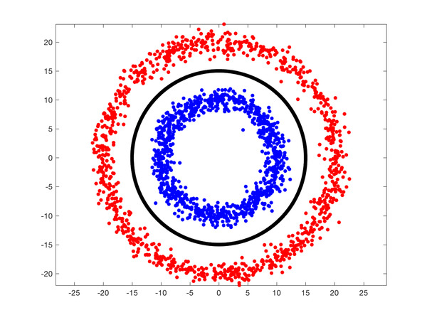
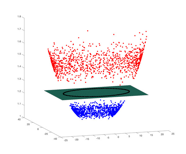
What if the data is not separable by a hyperplane? For example, in Figure 4, the two classes represented by the red and blue dots are not linearly separable. The decision boundary shown in black is actually circular.
In such a case, we use the Kernel Trick where we add a new dimension to existing data and if we are lucky, in the new space, the data is linearly separable. Let’s look at the Kernel Trick using an example.
In Figure 5, we have added a third dimension (z) to the data where,
![]()
The above expression is called a Gaussian Radial Basis Function or a Radial Basis Function with a Gaussian kernel. We can see the new 3D data is separable by the plane containing the black circle! The parameter ![]() controls the amount of stretching in the z direction.
controls the amount of stretching in the z direction.
In our next post in this sequence, we will learn how to use SVM in Python and C++ applications.









100K+ Learners
Join Free OpenCV Bootcamp3 Hours of Learning