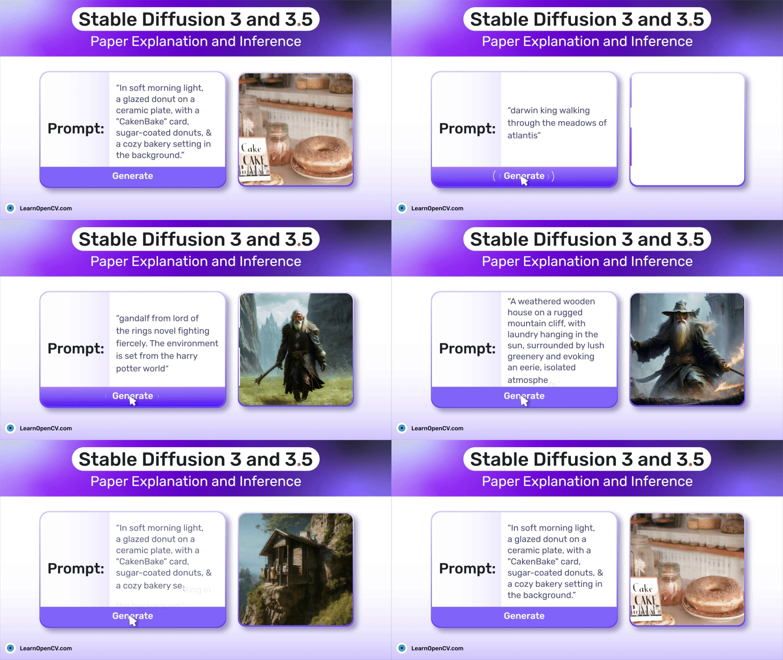
Stable Diffusion 3.5, released on June 2024 by Stability AI, is the third iteration in the Stable Diffusion family. The Turbo-Large and Large variants of the SD3.5 family are Stability AI’s most advanced text-to-image open-source models yet. Stability AI has recently collaborated with ARM to produce on-device generative audio in smartphones.

These models are based on the fundamental concept of latent diffusion(even used in text-to-video diffusion models), which we will cover later in this article before getting acquainted with the concepts of SD3.5.

This article provides an intuitive understanding of how Stable Diffusion 3.5 works. We have provided an Inference script of the Stable Diffusion 3.5 Large Turbo model at the end of this article. Before proceeding any further, let’s take a moment to understand Diffusion Models.

Defining Diffusion (and Variants) and the Reason for this Nomenclature
1. Latent Diffusion
Stable Diffusion
Inference with Stable Diffusion 3.5 Large Turbo, Large and Medium
Comparison of Stable Diffusion 3.5 Large Turbo and Flux Schnell
Conclusion
References

What is diffusion, and how does it work?

Diffusion Space, Image Manifold Space and Denoised Interpolation — *Fig 1: Diffusion Process Space*

Diffusion in classical mechanics refers to the transfer of particles—or any tangible quantity—from an area of high concentration to an area of low concentration. Inspired by this concept, the authors of Denoising Diffusion Probabilistic Models (DDPM) introduce noise into a target image (which has very low noise) to align it with the noise data distribution. This process is known as Forward Diffusion, as described by the original authors of the diffusion paper. Conversely, the process is called Reverse Diffusion when the target data distribution is derived from this noisy image.

Diffusion Process describing Forward and Reverse Process — *Fig 2: Simple Diffusion Process*

The image above shows how the forward and reverse diffusion process works by representing it in probabilistic notations. However, these notations represent the data distributions at each timestamp. As we observe, the image becomes progressively noisier when we follow the path of $q(X_t \mid X_{t-1})$ . This indicates that noise is gradually diffusing into the target distribution. Essentially, our neural network will learn the noise distribution between two timestamps during the reverse diffusion process by regressing the mean and variance of the latter.

It is not always necessary to regress both central tendencies; we can instead focus solely on regressing the noise by simplifying the diffusion loss function.

Let’s take a look at how the authors have defined the algorithm for Denoising Diffusion Probabilistic Models (DDPM):

Denoising Diffusion Probabilitic Model Algorithm for Training and Sampling — *Fig 3: Simple Diffusion Algorithm*

Where,

$\[\begin{aligned}\\epsilon \rightarrow \text{Actual Noise} \\\epsilon_{\theta} \rightarrow \text{Predicted Noise} \\\mathcal{N}(0, \mathbf{I}) \rightarrow \text{Standard Normal Distribution} \\\alpha_t \rightarrow 1 - \beta_t \quad \text{(Variance Schedule or Scaling Factor)} \\\mathbf{z} \rightarrow \text{Vector from } \mathcal{N}(0, \mathbf{I}) \\\nabla_{\theta} \rightarrow \text{Divergence} \\\mathbf{x}_0, \mathbf{x}_T \rightarrow \text{Samples at time } t = 0 \text{ and } t = 1\end{aligned}]$

As mentioned, we can see that the model is trying to regress epsilon (parameterized by $\theta$ ) by getting as close to the original noise as possible.

Now that we know the algorithm guiding the diffusion process, we can move to understanding Latent Diffusion Models(LDM).

Latent Diffusion

Compared to Vanilla Diffusion, Latent Diffusion incorporates one key change that makes it more applicable to real-life scenarios. This idea is derived from the models used in Variational Autoencoders (VAEs).

The latent variable ‘Z’ is a low-dimensional representation of the original data. This representation is beneficial for generation, as it captures the essential attributes of the data without any extraneous information. This vector encapsulates everything needed to reconstruct the original distribution using VAEs.

When generating our target distribution from noise, we utilize a significant amount of resources; in fact, diffusion (considering both forward and reverse diffusion processes) is resource-intensive. To address this issue, we can apply the concept of latent spaces from Variational Autoencoders (VAEs).

Firstly, a VAE encodes the target data into a latent space, resulting in a less complex, lower-dimensional representation than the original target distribution. Consequently, applying a diffusion framework or model to this latent vector makes the reverse process more efficient and faster.

Now, let’s take a look at the architecture of latent diffusion models:

Latent Diffusion Model Architecture — *Fig 4: LDM Architecture*

The authors of the DDPM paper employed a U-Net architecture as a neural network for the diffusion process, which has since become a standard for diffusion neural networks. This architecture offers several advantages for our purposes, including multi-scale feature extraction, versatility with conditional inputs, and efficient memory and computational usage.

As we can see in the image, a section named Conditioning. It refers to the process in which the generation of sample images adheres to the instructions provided in the condition itself, or you can say the prompt provided by the user, rather than just being a random prediction from the diffusion model. This conditioning can take various forms, such as semantic maps, text, or images.

With a foundational understanding of diffusion and latent diffusion models, it’s time to introduce Stable Diffusion.

Stable Diffusion 3.5

Before understanding Stable Diffusion, we must know what flow matching means.

Ordinary Differential Equation Solver for Stable Diffusion 3. Flow of ODE. — *Fig 5: ODE paths for SD3*

Flow Matching for Stable Diffusion 3.5

The dotted lines shown in the figure above represent what is known as “flow.” This concept describes how a sample point from the latent space distribution transforms into a component of the target distribution. This may seem a bit ambiguous and difficult to grasp at first, but by the end of this section, a clear understanding of how flow matching works and its relation to Stable Diffusion will be established.

Specifically, the paper’s authors introduced flow matching as a simple and intuitive training objective aimed at regressing onto a target vector field that produces a desired probability path. A probability path refers to the route that a particular distribution (in our case, the noise distribution) takes to achieve the state of another distribution. Assuming intermediate knowledge of matrices and determinants, this process resembles the row-wise(or column-wise) matrix transformation.

Simulation of ODE. Path Traversal simulation for SD3. — *Fig 6: ODE path traversal simulation in SD3*

All in all, we can say that flow matching or normalizing flow transforms a simple distribution ( gaussian distribution ) into a complex one by applying a series of invertible transformation functions.

Let’s go further into this concept by introducing some mathematical details.

FM Objective:

Fig 7: $Vt$ and $Ut$ are vector fields of a single point pointing towards a particular direction to move

The above expression is a simple mean square error formula between two vector fields. This equation regresses the vector field $V_t$ , which is parameterized by $\theta$ , and ultimately aims to reach a known vector field $U_t$ . However, the challenge we face is that we do not have any information about what the final vector field $V_t$ looks like. Additionally, the objective presented is impractical to use because we lack prior knowledge of what appropriate distributions $P_t$ , and $U_t$ , should be.

To address this, we need to get acquainted with mathematics to make it more intuitive to understand how to arrive at the final probability distribution or target image. This is where Conditional Flow Matching (CFM) comes into play.

Fig 8: CFM Objective

The authors have demonstrated that optimizing the Conditional Flow Matching (CFM) objective is analogous to optimizing the Flow Matching (FM) objective. This effectively indicates that the divergence of the loss function for flow matching is nearly equal to the divergence of the loss function for conditional flow matching.

Since we do not have a straightforward method for obtaining $U_t$ ,, we will transform it into another representation.

Before proceeding, let’s define a few concepts: a probability path and a vector field are distinct entities. A vector field assigns a vector to every point in space, while a path specifies a vector for only a subset of points that follow a particular curve (in our case, this will be a Gaussian curve). Assuming each path takes the form of a Gaussian, we can express it according to the equation shown below:

Fig 9: Assumed Probability path for Conditional Flow Matching

Now, let’s move on these paths. Mathematically, it means shifting the mean of our data point to a new position and then scaling it with a standard deviation.
Mathematically showing how this point moves over time, we can use the push-forward equation and substitute these values in our original CFM loss; we get something like this:

Re parameterized equation of flow matching for tractability using Push Forward Method. — *Fig 10: Re parameterized Conditional Flow Matching*

In the equations above, $\psi$ represents a function that defines the transformation of each point.

As the authors explore the optimal mean and standard deviation over time for transforming a point towards the target point, they deduced (through induction alone) that the Optimal Transport method—characterized by a linear or straight flow—is the most effective approach to achieving the ultimate goal of reaching the final target distribution.

The final loss function for the Optimal Transport method is formulated as follows:

Final Conditioned Flow Matching Objective or Loss Function — Fig 11: Final CFM loss Equation

Comparison between flow of simple diffusion and optimal transport optimized flow diffusion in SD3 — *Fig 12: Simple Diffusion flow v/s SD3 Flow*

As visible in the image shown above, the way a diffusion model travels towards the target distribution and flow matching approaches are quite different. The paper’s authors showed that the Optimal Transport function for flow matching is the best practice for producing the most accurate samples in optimal time complexity.

Timestamp Sampling used in Stable Diffusion 3.5

Finally, we have arrived at the last concept to understand the Stable Diffusion 3.5 model. A Stable Diffusion 3 model is essentially a refinement of the diffusion model, enhanced by adding flow matching and timestamp sampling techniques. The previous discussion outlined how flow matching integrates into the diffusion process to ensure the shortest and most optimal path.

Until now, all our timestamps have been equally weighted and derived from a uniform distribution. However, as noted by the authors of the Stable Diffusion 3 paper, the differences between intermediate timestamps tend to be more significant than those at the beginning or end. Thus, it is essential to incorporate a weighted loss function that assigns greater importance to the intermediate timestamps.

In their research on timestamp sampling techniques, the authors concluded that Logit-Normal Sampling would yield the most optimal results.

In summary, we can say that:

Diffusion + Rectified Flow (Flow Matching) + Logit-Normal Sampling leads us to Stable Diffusion 3.5.

The architecture of Stable Diffusion 3.5

The architecture is based on the Diffusion Transformers model, utilizing an Encoder (VAE) to generate noise latent variables, similar to the MMDiT architecture. It also includes a decoder(VAE) to upscale the output of our model.

Let’s begin with the first layer, where captions (textual prompts) are processed and transformed into embeddings within an embedding space.

Textual Embedding

Based on Stable Diffusion 3, MMDiT employs three textual encoders: CLIP-G/14, CLIP-L/14, and a T5 XXL encoder with approximately 5 billion parameters. The rationale behind using these three textual encoders is to enhance performance. This configuration offers flexibility during inference, allowing us to balance model performance and memory efficiency by removing the T5 XXL encoder if desired.

We have the option to include the T5 XXL encoder during inference. Removing this encoder helps reduce memory consumption with only a minimal loss in accuracy. When the T5 XXL encoder is removed, its output becomes a tensor of zeros.

The simplified code appears as follows:

Code Snippet of defining text_encoders of SD3, particularly T5 XXL. — *Fig 13: T5 XXL inclusion/removal code snippet*

Patchify

As the pooled text representations retain only coarse-grained information about the textual input, the network also needs insights from the sequence representation. To achieve this, we create patch encodings by flattening 2×2 patches and adding positional encodings. We then concatenate this with text encodings, ensuring both have the same dimensionality.

The factor by which we scale down our image (referred to as patch_number) depends on the scale factor, as shown in the image below:

Code Snippet of Patch Generation function on latent image space — *Fig 14: Patchification of latent image code snippet*

DiT backbone used in Stable Diffusion 3.5

After the above two procedures, the MM-DiT model follows the DiT backbone and applies a sequence of Modulated Attention and MLP layers.

To best understand the upgrade MM-DiT brought against vanilla DiT, we can summarize it in one sentence: DiT is the special case of MM-DiT with only one set of shared weights for all modalities.

Stable Diffusion 3.5 Architecture — *Fig 15: SD 3.0 Architecture*

Simplified Stable Diffusion 3.5 Architecture. Modulated Attention Mechanism — *Fig 16: Simplified SD3.0 Architecture*

One question you might ask after seeing the architecture is what alpha, beta, and gamma represent.

The answer lies in the way diffusion transformers implement attention mechanisms. The attention mechanism they use is modulated attention, as seen in the simplified architecture image.

Code Snippet of Modulation function used in Stable Diffusion 3/3.5 for attention mechanism — *Fig 17: Modulated Attention Mechanism as shown in the image above*

The input vector, which includes the skip connection input, can be expressed as input vector + (input * scale) + shift. Scales and shifts refer to alpha, beta, and gamma parameters visible in the model architecture.

Like DiT, MMDiT employs adaptive layer normalization (adaLN) instead of traditional layer normalization (LN). The authors of the DiT paper explain that adaLN is the most compute-friendly option. Additionally, it is the only conditioning mechanism that applies the same function uniformly across all tokens.

Adaptive Layer Normalization or adaLN function used in Stable Diffusion 3.5 source code. — *Fig 18: Layer Normalization used in SD3.5 and DiT is adaptive Layer Normalization or adaLN*

Lastly, the authors discussed the separate sets of weights they used to understand the complexity of each modality individually. This approach is equivalent to having two transformers, one for each modality. While it might seem that this would lead to no correlation between the two modalities, combining both sequences for the joint attention operation addresses this issue.

Additionally, the architecture presented differs from the original MMDiT architecture by incorporating more self-attention blocks. This modification pertains to the Stable Diffusion 3.5 medium (MM-DiTx), a 2.5 billion parameter model. Because of this lower parameter count, it is less accurate; thus, the authors introduced additional layers of attention to enhance its ability to understand the relationships and semantic meanings within the sequences.

MM-DiTx (Stable Diffusion 3.5 medium ~2.5 B parameter) architecture — *Fig 19: MMDiTx Architecture or SD3.5 medium*

To better understand a model’s way of calculating noise and outputting a sample, we should look at a snippet of the model’s pipeline where it regresses noise.

Reverse Diffusion Process or Denoising Algorithm Implementation as described in source code of Stable Diffusion 3.5 — *Fig 20: Denoising Algorithm(Reverse Diffusion Process) of SD3.5 code snippet*

Here, we can see that inside the denoising loop, the transformer model gives predicted noise as output, which is then chunked to generate two noises: predicted unconditional noise and predicted textual noise. Finally, latent(t-1) is generated using the scheduler and latent from the previous (t) timestamp.

Inference with Stable Diffusion 3.5 Large Turbo, Large, Medium

Hardware or GPU requirements for each Stable Diffusion 3.5 model along with GPU requirements for FLUX models also. — *Fig 21: Hardware Requirements for various SD models*

Download Code To easily follow along this tutorial, please download code by clicking on the button below. It's FREE!

Click here to download the source code to this post

In the image above, Stability AI has outlined the compatibility of various models with different GPU architectures.

Next, let’s explore the inference process and closely examine the inference script.

Before we proceed, let’s look at GPU consumption and usage during the inference process. We have set up an instance with one A6000 GPU with a maximum memory capacity of 48GB.

Nvidia A6000 GPU usage and Consumption in inferencing Stable Diffusion 3.5 Large Turbo — *Fig 22: Single Nvidia GPU A6000 Consumption and Usage*

Following are the dependencies(like diffusers) that we need to install for the Stable Diffusion 3.5 Large Turbo module.

!pip install -U diffusers
!pip install transformers
!pip install accelerate
!pip install sentencepiece
!pip install protobuf

Next, we import the necessary functions and create a pipeline for our Stable Diffusion 3.5 Large Turbo Model, which only requires the Model ID and Torch Dtype as arguments.

import torch
from diffusers import StableDiffusion3Pipeline

Now, let’s create an instance of Pipeline and call Stable Diffusion 3.5 Large Turbo Model.

pipe = StableDiffusion3Pipeline.from_pretrained("stabilityai/stable-diffusion-3.5-large-turbo", torch_dtype = torch.bfloat16)

pipe = pipe.to("cuda")

A manual seed is defined to ensure that every time we run the sample.

The Number of Inference Steps: Intermediate Latents are generated before reaching the final output.
The Guidance Scale: The degree to which we want our model to adhere to the prompt. A value of 0 means the model will generate a sample based on the prompt but will be flexible in its generation, thereby not strictly adhering to it.

Finally, let us use the pipeline instance to create our synthesized image of a Capybara.

torch.manual_seed(1)
image = pipe("cute capybara holding a card on which 'HELLO WORLD' is written", num_inference_steps = 30, guidance_scale = 0.0).images[0]

image.save("capybara.png")

Sample Image of a Capybara generated from Stable Diffusion 3.5 Large Turbo — *Fig 23: Capybara sample image*

Comparison of Stable Diffusion 3.5 Large Turbo and Flux Schnell

Model similarities and differences overview

The Flux Schnell model is a 12B parameter model, whereas the SD3.5 large-turbo model is an 8.1B parameter model.
Typically, the number of inference steps for Flux Schnell ranges between 3-6; for SD3.5 large-turbo, it’s fixed to 20.
The Guidance Scale for both models is set to 0. However, the Flux Schnell model does not explicitly require a guidance scale parameter in its pipeline.
When a pipeline is instantiated, we can define another parameter called ‘negative prompt.’ This tells an AI diffusion model to avoid generating specific elements or characteristics in its output. The vital thing to notice is that the Flux Schnell model is not designed to provide negative prompts in its pipeline. At the same time, in Stable Diffusion 3.5, users can pass this parameter if they want the model to avoid certain practices while generating a sample.
If you are interested to know more about Flux models, do visit our another article Flux Image Generation.

vincent van gogh's starry night painting artistic style generation with Batman modification — Fig 24: Batman in Starry Night art by **Van Gogh**

Red-Green color dragon set in a cloudy and mountainous place style generation — *Fig 25 Dragon with green wings in a cloudy and mountainous place*

Portrait of a woman giving talk and working at Google tech style generation — *Fig 26: Portrait of a woman at Google tech conference*

mona lisa original portrait style generation — *Fig 27: **Mona Lisa** by Da Vinci*

Conclusion

This article takes a walk through a wide variety of concepts like latent diffusion, flow matching, etc., in a very informative manner, covering final loss mathematical equations, elaborative explanations of code blocks, etc.

To summarize this article, we covered:

Diffusion and its Training and Sampling Algorithm.
Latent Diffusion Models and their Architecture.
Probability Path and Flow Matching.
The most efficient path for diffusion models to follow.
Stable Diffusion models and their architecture.
Inference code blocks.
Sample comparison between Flux Schnell and SD3.5 Large Turbo.

Generative AI has opened up many research opportunities, especially diffusion models, as their practical applications keep increasing daily, ranging from commercial content creation to artistic innovation.

Happy Learning 🙂

Stable Diffusion 3.5: Paper Explanation and Inference

What is diffusion, and how does it work?

Latent Diffusion

Stable Diffusion 3.5

Flow Matching for Stable Diffusion 3.5

Timestamp Sampling used in Stable Diffusion 3.5

The architecture of Stable Diffusion 3.5

Textual Embedding

Patchify

DiT backbone used in Stable Diffusion 3.5

Inference with Stable Diffusion 3.5 Large Turbo, Large, Medium

Comparison of Stable Diffusion 3.5 Large Turbo and Flux Schnell

Conclusion

References

Get Started with OpenCV

Subscribe to receive the download link, receive updates, and be notified of bug fixes

Which email should I send you the download link?

What is diffusion, and how does it work?

Latent Diffusion

Stable Diffusion 3.5

Flow Matching for Stable Diffusion 3.5

Timestamp Sampling used in Stable Diffusion 3.5

The architecture of Stable Diffusion 3.5

Textual Embedding

Patchify

DiT backbone used in Stable Diffusion 3.5

Inference with Stable Diffusion 3.5 Large Turbo, Large, Medium

Comparison of Stable Diffusion 3.5 Large Turbo and Flux Schnell

Conclusion

References

Subscribe & Download Code

Get Started with OpenCV

Subscribe to receive the download link, receive updates, and be notified of bug fixes

Which email should I send you the download link?