Exploring DINO: Self-Supervised Transformers for Road Segmentation with ResNet50 and U-Net

DINO is a self-supervised learning (SSL) framework that uses the Vision Transformer (ViT) as it’s core architecture. While SSL initially gained popularity through its use in natural language processing (NLP) tasks, it has also made significant progress in the field of computer vision. Self-Supervised Learning (SSL) serves as an alternative pre-training strategy, that doesn’t relay on labelled data. One notable development in this area is the DINO(Distillation with No Labels), a model by Facebook AI, with a new and improved version, DINOv2, being introduced last year.

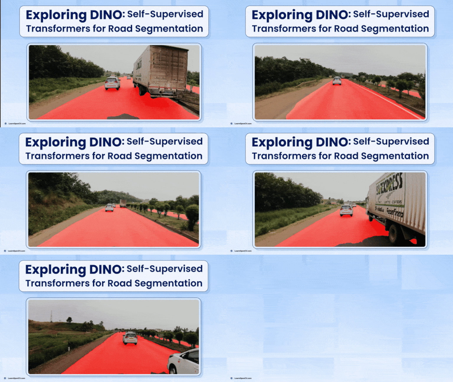
In this article, we we take an in-depth look into the history of Self-Supervised Learning, followed by DINO a self-supervised learning model, and its internal workings, finally we fine-tune a DINO-based ResNet-50 backbone for a downstream segmentation task—specifically for Indian road segmentation on the IDD dataset. We achieve IOU of 0.95 when training the DINO-ResNet50 Unet model. We’ll cover the following key topics:

• What is Self-Supervised Learning (SSL) and its historical background?
• What is DINO and how does it work?
• How to fine-tune DINO for downstream road segmentation task?

1. What is Self-Supervised Learning (SSL)?
2. DINO Paper Explained
   1. Momentum Encoder
   2. Multi-Crop Method
   3. DINO Internal Working
   4. Mode Collapse
      1. Uniform Distribution Output
      2. One Class Domination Output
   5. DINO: A Powerful Multi-Purpose Model
   6. DINO Pseudo code Explanation w/o Multi-crop
3. Road Segmentation using DINO Resnet-50 Unet
   1. Custom Dataset Class
   2. Model Building
   3. Training and Validation Loop
   4. Inference

Click here to download the source code to this post

What is Self-Supervised Learning (SSL)?

From a broader perspective, machine learning can be divided into three main sub-fields:

• Supervised Learning
• Unsupervised Learning
• Reinforcement Learning

Within unsupervised learning, there are two types of models:

• Generative Models
• Self-Supervised Models

In this article, we will focus on the second type: self-supervised models.

In general, when data comes with labels, it’s called supervised learning, and when there are no labels, it’s referred to as unsupervised learning. Since self-supervised learning falls under the unsupervised category, models are typically trained on unlabeled data. These models help generate valuable feature representations by solving pretext tasks, which are designed to learn meaningful features directly from the data.

Around 2010, there was a lot of excitement around AI, but a gap between expectations and reality remained. In both academic and industrial research, deploying AI models to solve real-world problems was still a distant goal. However, after the success of models like GPT-3 and BERT, many researchers began to see self-supervised learning as a way to bridge this gap. For a long time, supervised training was considered the only way to achieve strong model performance, largely due to the impact of the ImageNet moment and the success of AlexNet. But since labeled data is hard to obtain—and creating labeled datasets is both costly and time-consuming—self-supervised learning with unlabelled data pre training has emerged as a promising alternative.

Meta’s research team, along with Yann LeCun, has long been strong advocates for self-supervised learning. LeCun famously described the modern training paradigm using the now well-known “cake analogy” during his 2016 NIPS keynote. According to him:

“If intelligence is a cake, the bulk of the cake is unsupervised learning, the icing on the cake is supervised learning, and the cherry on the cake is reinforcement learning (RL).”

LeCun updated his cake recipe at the 2019 International Solid-State Circuits Conference (ISSCC) in San Francisco, replacing “unsupervised learning” with “self-supervised learning”. And if you observe carefully, this is the same procedure how ChatGPT was trained. First it was pre trained on the entire internet data and then followed by a supervised fine-tuning stage and finally the RLHF which used the smallest amount of data. 

In terms of NLP, self-supervised learning got a lot of success although there had been attempts to make CNNs work on a self-supervised framework but after the vision transformer came to the picture, computer vision saw the true success in self-supervised paradigm. Self-supervised Computer Vision techniques are more of a bag of tricks and different training methods rather than involving heavy maths. Methods like: 

• Masked encoders are scalable vision learners, where you are given a masked out image (70-75% masking), and pass the unmasked image patches through the ViT encoder and the full image is retrieved through the decoder part. The concept is similar to next token prediction, or masked token prediction. taking up strategies from NLP.

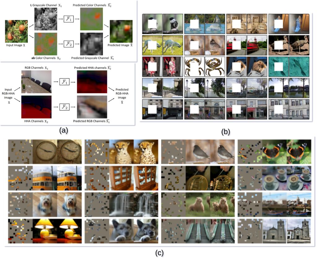
• Similar work has been done, where instead of filling up the masked out regions, the task was to colourise a grayscale image, or given a single channel predicting the rest of the channels (LAB, RGB etc.).
• After that the concept of contrastive learning methods came in, where the main concept was, distance between the feature representation of similar image should be small, and distance between dissimilar images should be larger in a n dimensional feature space. Like given an image of a dog, and a cropped out image of a dog should be closer that the image of the dog and a couch. The model should be able to figure out this concept without the labelled information.

One of the groundbreaking self-supervised computer vision work using vision transformer work is DINO. We will be mostly talking about DINO in this article, and how the DINO backbone can be used for downstream tasks, such as road segmentation.

DINO Self-Supervised Learning: Paper Explained

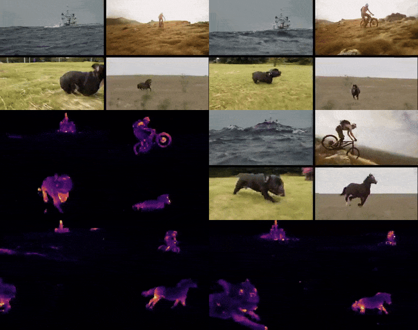
DINO stands for Distillation with No Labels, and it uses a self-supervised approach where the model learns to generate good representation without needing explicit labels. DINO has a student teacher model, in a general knowledge distillation kind of setup. Generally in knowledge distillation, you have a large model which you got from training the model on a large set of data, and you want a small version of the model. To do so, you use the bigger model and the same dataset to train a smaller model; this is called knowledge distillation. This approach particularly works better than training the smaller model from scratch. But, as in DINO, there is no pre-trained teacher, there is only a student that is getting updated and based on that the teacher parameters are being updated.

The effectiveness of DINO relies on few things,

• Momentum Encoder
• Multi-corp Training

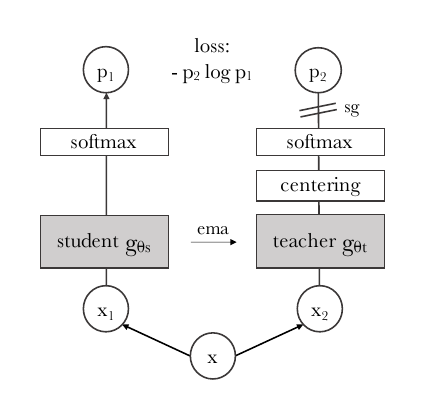
Above is the Student teacher model of DINO, the input x is augmented to generate and . is fed to the student model and the is fed to the teacher model, after passing through the teacher model the output is centered and sharpened to output a fixed size vector . Both student and teacher networks output a size vector. These two vectors with a cross-entropy loss are used to calculate the distance. We update the teacher’s parameters gradually using an exponential moving average (EMA) of the student network’s parameters. To ensure this, we apply a stop-gradient (sg) operator on the teacher, allowing gradients to flow only through the student network during training. This way, the teacher evolves smoothly without directly receiving gradients.

There are few things that needs to be highlighted, such as,

Momentum Encoder

Momentum Encoder is nothing but the method used to update the teacher model parameters, by using Exponential Moving Average. Below equation takes the current parameters of the teacher model, and the updated student parameter model, to calculated the new weights for the teacher model,

• are the teacher network parameters.
• are the student network parameters.
• is the momentum coefficient (or decay rate), typically close to 1 (e.g., 0.999) to ensure that the teacher network evolves slowly.

The momentum encoder ensures that the teacher network is more stable and consistent than the student network, which allows the student to learn better representations by trying to match a slowly evolving target, reducing fluctuations in the learning process.

The teacher in DINO performs a type of model ensembling similar to Polyak-Ruppert averaging, which involves averaging the weights of a model over time with an exponential decay. This technique smooths out model updates and reduces fluctuations, leading to more consistent learning and better overall performance.

Multi-Crop Method

In other self-supervised frameworks, generally a positive image pair and a negative image pair is created, and the framework loss is designed such a way, that the distance between the positive pairs are high and distance between the negative pairs are low, and if a model trained using this framework can show these properties then it can be assumed that the model has a good representation of the data.

In DINO on the other hand, the multi-crop method is used for model training. In multi-crop global and local crops are generated, global crops are the crops that have >50%  of the image, and local crops are the crops that have <50% of the image. If the same object appears in both the crops then the student model needs to output the K dimensional vector, that is closed/similar to the teacher model’s K dimensional vector, as the goal is to predict the same representation. 

DINO Internal Working

Cross-entropy after softmax is like assigning images to soft clusters. The softmax outputs a K dimensional vector, representing probabilities for K classes, Then, cross-entropy loss is used to compare the predicted probability distribution with the ground truth labels, guiding the model to classify inputs into one of the predefined classes (hard assignment). In DINO the model is trained in a way that the softmax can be interpreted as assigning each input to a soft cluster.

Mode Collapse

There are two types of mode collapse that the DINO paper talks about. 

Uniform Distribution Output

The output of the softmax, the K dimensional vector, has all values the same, which means that the output probabilities are evenly spread across all possible classes, which is equivalent to making random predictions.

One Class Domination Output

In this case, the model’s output is concentrated on just one dimension, meaning the model predicts one specific class with absolute certainty, regardless of the input. Essentially, the output is highly imbalanced and dominated by a single class.

Centering and Sharpening is used to stabilize the model output, centering helps in One dimension domination issue, where sharpening helps with the Uniform distribution  issue.

DINO: A Powerful Multi-Purpose Model

Below are the few example where the DINO model can be used,

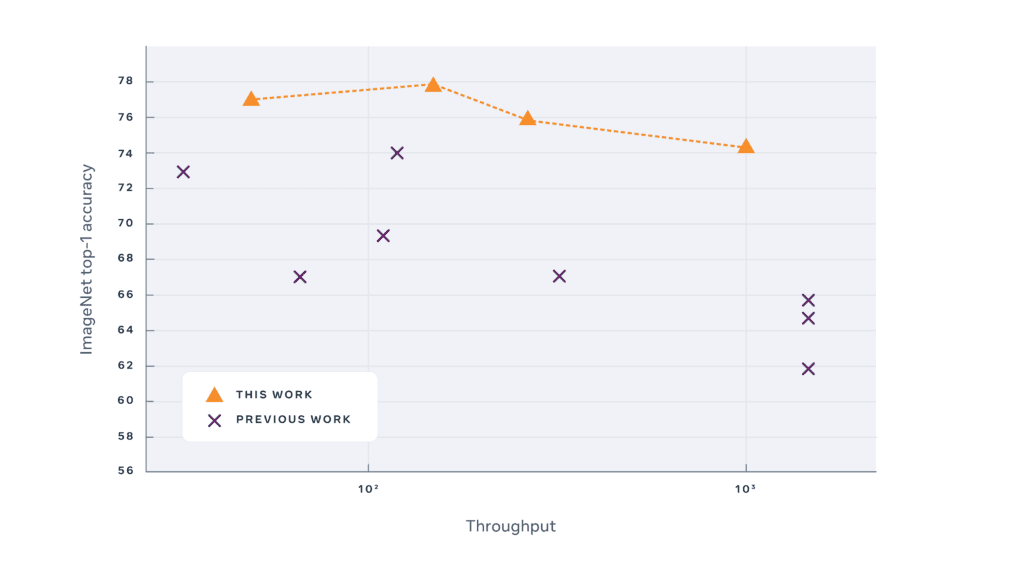
• Classification: DINO can be used for downstream tasks like classification. The authors found out that the feature map was providing attention to the subject of interest, without being trained to do so.These rich features can be used with KNN classifiers to do classification. DINO achieves 80.1% top-1 on ImageNet in linear evaluation with ViT-Base.

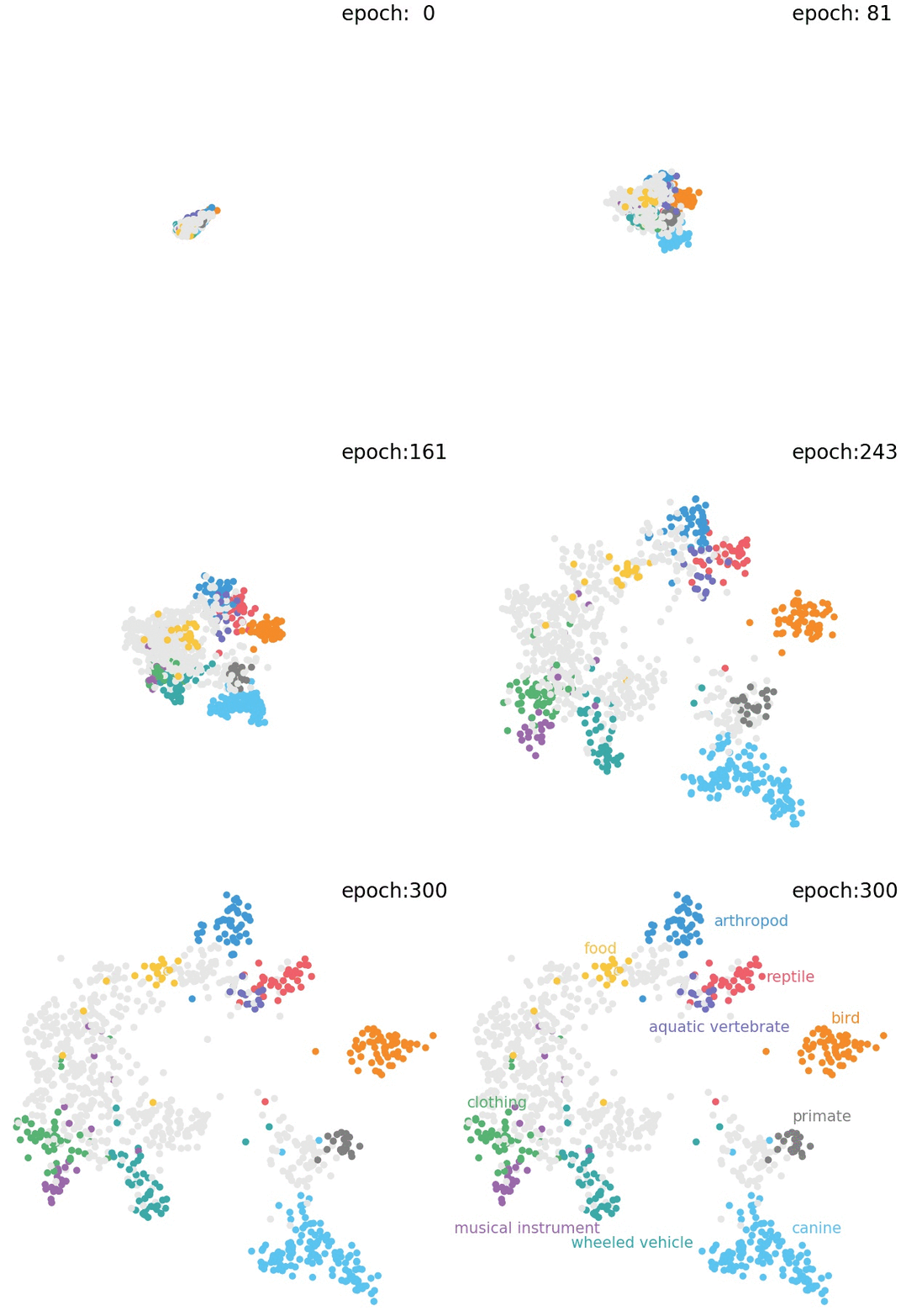
• Clustering: DINO has a deep understanding of the visual world by identifying object parts and common traits across different images. The model develops a feature space with an intriguing structure, where, for instance, animal species are distinctly grouped in a way that mirrors biological taxonomy.

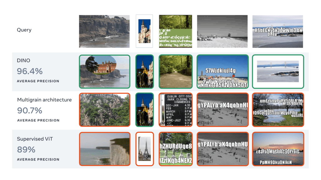
• Image Retrieval: The authors found that when they are training on imagenet it is able to cluster the images under the same class, in the feature space. Not only that but it also clusters the similar classes with each other. This can be used for Image retrieval or copy detection.

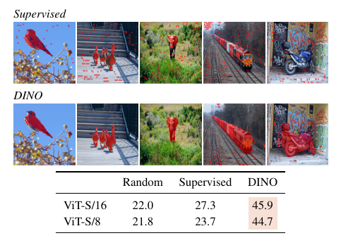
• Image Segmentation: The DINO feature map looks like a segmentation map, without being trained to do so. They test their model on DAVIS 2017 video object segmentation. It manages to track and segment objects  at the same time across frames.

DINO Pseudo code Explanation w/o Multi-crop

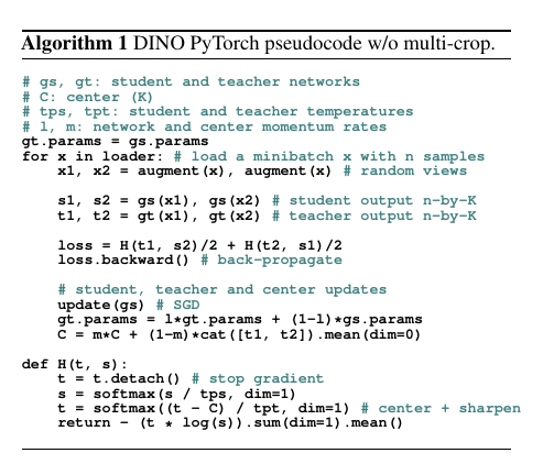
Given an image x it generates x1 and x2 using augmentation, both x1 and x2 are sent to the student model gs, to generate s1, s2 and also sent to the teacher model gt to generate t1, t2. These t1, s2 and t2, s1 are used to calculate the cross entropy loss. This loss is an average of the student’s output matching the teacher’s output, considering the two augmented views. This comparison encourages the student to learn meaningful features similar to the teacher’s. update(gs) updates the student parameter, when the teacher parameter updates using EMA. The center C is updated using a similar moving average of the teacher’s output. This center is used to stabilize the training and avoid collapse by ensuring the teacher’s output doesn’t collapse to a single mode. In the H function, the teacher’s output is centered and sharpened by subtracting C and applying softmax.

Road Segmentation using DINO Resnet-50 Unet

The idea here is to use one of the pretrained backbone trained using DINO self-supervised framework, and use it with Unet to do Road segmentation using the IDD dataset. Here we have decided to use the ResNet-50 backbone with Unet for this segmentation task. Let’s go through the code step by step. Generally, there are 4 main steps,

• Custom Dataset Class
• Model Building
• Training and Validation Loop
• Model Inference 

Below is an inference example of the DINO downstream Road Segmentation task,

Custom Dataset Class

Generally in Pytorch we create a dataset class, where we define, given an index, how we upload the image and mask associated with that index. But before we do that we need to download the IDD dataset.

Download and Prepare IDD Segmentation Dataset:

To start, we’ll download Part 1 of the segmentation dataset. Follow this link to download the IDD dataset. Before downloading, you’ll need to create an account using your credentials. The dataset consist of 1k validation, 7k training and 2k test images with annotations stored in json format. We will first turn the json annotations to png images with color coding. For doing the annotation format conversion use the below command,

$ python public-code/preperation/createLabels.py --datadir idd-segmentation/IDD_Segmentation/

Now if you checkout any folder inside /gtFine/train/ you will find the images. 

Now that we are done preparing the dataset, let’s write the dataset class and dataloader,

class RoadsDataset(torch.utils.data.Dataset):

    """Indian Driving Dataset. Read images, apply augmentation and preprocessing transformations.
    
    Args:
        df (pandas.DataFrame): train or validation data frame
        class_rgb_values (list): RGB values of select classes to extract from segmentation mask
        augmentation (albumentations.Compose): data transfromation pipeline 
            (e.g. flip, scale, etc.)
        preprocessing (albumentations.Compose): data preprocessing 
            (e.g. noralization, shape manipulation, etc.)
    
    """
    
    def __init__(
            self, 
            df,
            class_rgb_values=None, 
            augmentation=None, 
            preprocessing=None,
    ):
        self.df = df
        self.image_paths = sorted([get_data_path(i) for i in self.df["image"].tolist()])
        self.mask_paths = sorted([get_data_path(i) for i in self.df["mask"].tolist()])

        self.class_rgb_values = class_rgb_values
        self.augmentation = augmentation
        self.preprocessing = preprocessing
    
    def __getitem__(self, i):
        
        # read images and masks
        image = cv2.cvtColor(cv2.imread(self.image_paths[i]), cv2.COLOR_BGR2RGB)
        # mask = cv2.cvtColor(cv2.imread(self.mask_paths[i]), cv2.COLOR_BGR2RGB) 
        mask = cv2.cvtColor(cv2.imread(self.mask_paths[i]), cv2.COLOR_BGR2GRAY) 
        

        mask = mask.astype('long') / 255.




        # apply augmentations
        if self.augmentation:
            sample = self.augmentation(image=image, mask=mask)
            image, mask = sample['image'], sample['mask']
        
        # apply preprocessing
        if self.preprocessing:
            sample = self.preprocessing(image=image, mask=mask)
            image, mask = sample['image'], sample['mask']

        
        return image, mask
        
    def __len__(self):
        # return length of 
        return len(self.image_paths)

This RoadsDataset class is a PyTorch Dataset used for loading and preprocessing images and segmentation masks from the Indian Driving Dataset.

• Initialization: Takes a DataFrame with image and mask file paths, along with optional class RGB values, augmentation, and preprocessing functions.
• __getitem__: Reads the image and corresponding grayscale mask, optionally applies augmentations and preprocessing, and returns the processed image and mask.
• __len__: Returns the length of the dataset based on the number of image paths.

The dataset is designed to support transformations like augmentation and preprocessing for efficient training. After the dataset class is created we pass the train and validation dataset class instances to the DataLoader to create the train and validation dataloader. The num_workers argument is very important because there you mention the number of CPU cores, the num_workers argument is crucial because it determines the number of subprocesses used for loading data in parallel during training. A higher number can speed up data loading, but if you set it too low, the data might not be fed into the model fast enough, slowing down training. 

# Get train and val dataset instances
train_dataset = RoadsDataset(
    train_df, 
    augmentation=get_training_augmentation(),
    preprocessing=get_preprocessing(preprocessing_fn),
    class_rgb_values=select_class_rgb_values,
)

valid_dataset = RoadsDataset(
    val_df,
    augmentation=get_validation_augmentation(), 
    preprocessing=get_preprocessing(preprocessing_fn),
    class_rgb_values=select_class_rgb_values,
)

# Get train and val data loaders
train_loader = DataLoader(train_dataset, batch_size=8, shuffle=True, num_workers=4)
valid_loader = DataLoader(valid_dataset, batch_size=1, shuffle=False, num_workers=4)

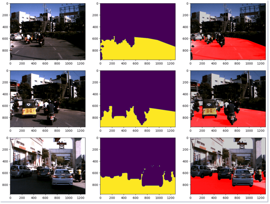
After the dataloaders are created we are done with the data pipeline, and we can move on to more interesting parts of the model building.

Model Building

class Conv2dReLU(nn.Module):
    def __init__(self, in_channels, out_channels, kernel_size=3, padding=1):
        super(Conv2dReLU, self).__init__()
        self.block = nn.Sequential(
            nn.Conv2d(in_channels, out_channels, kernel_size=kernel_size, padding=padding, bias=False),
            nn.BatchNorm2d(out_channels),
            nn.ReLU(inplace=True)
        )
    
    def forward(self, x):
        return self.block(x)

class DecoderBlock(nn.Module):
    def __init__(self, in_channels, out_channels):
        super(DecoderBlock, self).__init__()
        self.conv1 = Conv2dReLU(in_channels, out_channels)
        self.conv2 = Conv2dReLU(out_channels, out_channels)
        self.up = nn.Upsample(scale_factor=2, mode='bilinear', align_corners=True)
    
    def forward(self, x, skip):
        # Upsample
        x = self.up(x)
        
        # Resize skip connection to match the size of x
        if x.size() != skip.size():
            skip = F.interpolate(skip, size=x.shape[2:], mode='bilinear', align_corners=True)
        
        # Concatenate the skip connection (encoder output)
        x = torch.cat([x, skip], dim=1)
        
        # Apply convolutions
        x = self.conv1(x)
        x = self.conv2(x)
        return x

class UNetResNet50(nn.Module):
    def __init__(self, num_classes=2, pretrained=True):
        super(UNetResNet50, self).__init__()

        # Load ResNet50 pre-trained on ImageNet
#         self.encoder = models.resnet50(pretrained=pretrained)
        self.encoder = torch.hub.load('facebookresearch/dino:main', 'dino_resnet50')
        

        # Encoder layers from ResNet-50 (for skip connections)
        self.encoder_layers = [
            nn.Sequential(self.encoder.conv1, self.encoder.bn1, self.encoder.relu, self.encoder.maxpool),  # (64, H/4, W/4)
            self.encoder.layer1,  # (256, H/4, W/4)
            self.encoder.layer2,  # (512, H/8, W/8)
            self.encoder.layer3,  # (1024, H/16, W/16)
            self.encoder.layer4   # (2048, H/32, W/32)
        ]

        # Decoder (Upsampling blocks)
        self.decoder4 = DecoderBlock(2048 + 1024, 512)  # Block for layer4 + layer3
        self.decoder3 = DecoderBlock(512 + 512, 256)    # Block for layer3 + layer2
        self.decoder2 = DecoderBlock(256 + 256, 128)    # Block for layer2 + layer1
        self.decoder1 = DecoderBlock(128 + 64, 64)      # Block for layer1 + conv1

        # Final segmentation head
        self.segmentation_head = nn.Sequential(
            nn.Conv2d(64, num_classes, kernel_size=3, padding=1),
            # nn.Sigmoid()  # Use sigmoid for binary segmentation
        )

    def forward(self, x):
        # Save original input size for final upsampling
        original_size = x.shape[2:]  # (H, W)

        # Encoder forward pass
        x0 = self.encoder_layers[0](x)  # Initial convolution block (conv1)
        x1 = self.encoder_layers[1](x0)  # Skip connection 1 (layer1)
        x2 = self.encoder_layers[2](x1)  # Skip connection 2 (layer2)
        x3 = self.encoder_layers[3](x2)  # Skip connection 3 (layer3)
        x4 = self.encoder_layers[4](x3)  # Skip connection 4 (layer4)

        # Decoder forward pass
        x = self.decoder4(x4, x3)  # Decoder for layer4 + skip3
        x = self.decoder3(x, x2)   # Decoder for layer3 + skip2
        x = self.decoder2(x, x1)   # Decoder for layer2 + skip1
        x = self.decoder1(x, x0)    # Decoder for layer1 + initial conv1 output

        # Upsample the final output to match the input size dynamically
        x = F.interpolate(x, size=original_size, mode='bilinear', align_corners=True)

        # Final segmentation output
        x = self.segmentation_head(x)

        return x

# Example usage
if __name__ == "__main__":
    # Instantiate the model
    model = UNetResNet50(num_classes=2, pretrained=True)
    
    # Test the model with dummy input
    input_tensor = torch.rand(1, 3, 480, 640)  # Batch size 1, 3 channels (RGB), 480x640 image
    output = model(input_tensor)
    
    print(f"Output shape: {output.shape}")  # Should output (1, 2, 480, 640) for binary segmentation

The above model is the same as the ResNet50 with Unet segmentation head. ResNet50 here is used as an encoder backbone, and the decoder directly uses the different encoder downsample layer outputs. The Decoder is a Unet decoder which has upsampling implemented using nn.Upsample. It also concatenates the encoder output from the same level for better feature representation. More about the other blocks are explained below,

• Conv2dReLU Block: A helper block that performs a 2D convolution followed by batch normalization and ReLU activation. It’s used to simplify the process of creating convolution layers with ReLU activations in both the encoder and decoder.
• DecoderBlock: This block up-samples the input feature map using bilinear interpolation and concatenates it with the corresponding encoder feature map from the skip connections. It then applies two convolutional layers to refine the combined feature map.
• UNetResNet50:
  • ResNet50 as Encoder this U-Net uses a pre-trained ResNet50 (from DINO) as the encoder, which is being loaded as, torch.hub.load('facebookresearch/dino:main', 'dino_resnet50'). It extracts features from different stages (conv1, layer1, layer2, layer3, and layer4), which are used in the decoder. 
  • Skip Connections: The U-Net structure uses skip connections, which concatenate features from earlier encoder layers with the up-sampled decoder outputs. This helps retain high-resolution spatial information during up-sampling.
• Decoder: Each DecoderBlock up-samples the input and concatenates it with the corresponding encoder feature map. This combination is processed with convolutions to create a more detailed feature map for segmentation.
• Segmentation Head: After the final decoder block, a convolutional layer generates the final segmentation map, which has as many channels as the number of classes (num_classes).
• Upsampling: The model ensures that the final output has the same spatial resolution as the input image by using bilinear interpolation.
• Forward Method: During the forward pass, the input image is processed by the encoder and decoder. The skip connections are handled between corresponding encoder and decoder layers. Finally, the result is upsampled to match the original input size and passed through the segmentation head for output.

Training and Validation Loop

# define loss function
dice_loss = DiceLoss(mode='multiclass')
cross_entropy_loss = nn.CrossEntropyLoss()
loss_fn = lambda outputs, targets: dice_loss(outputs, targets) + cross_entropy_loss(outputs, targets)

# define metrics
iou_metric = torchmetrics.JaccardIndex(num_classes=2, task="multiclass").to(DEVICE)


# define optimizer
optimizer = torch.optim.Adam([dict(params=model.parameters(), lr=1e-4,  weight_decay=1e-5)])



# Sample training loop
def train_one_epoch(model, dataloader, optimizer, loss_fn, iou_metric, device):
    model.train()
    running_loss = 0.0
    running_iou = 0.0
    
    for images, masks in tqdm(dataloader):
        images, masks = images.to(device), masks.to(device)
        
        # Forward pass
        outputs = model(images)
        
        # Compute loss
        # print(outputs.shape, masks.squeeze(1).shape)
        loss = loss_fn(outputs, masks.squeeze(1))
        # loss = combined_loss(outputs, masks.squeeze(1))
        
        # Zero gradients, backpropagation, and optimization
        optimizer.zero_grad()
        loss.backward()
        optimizer.step()
        
        # Accumulate loss and IoU
        running_loss += loss.item()
#         running_iou += iou_metric(outputs, masks).item()
        # Compute IoU
        preds = torch.argmax(outputs, dim=1)
#         print(preds.shape, masks.squeeze(1).shape)
        running_iou += iou_metric(preds, masks.squeeze(1)).item()
    
    return running_loss / len(dataloader), running_iou / len(dataloader)



# Modified validation loop with visualization
def validate_one_epoch(model, dataloader, loss_fn, iou_metric, device, visualize=False, num_visualizations=2):
    model.eval()
    val_loss = 0.0
    val_iou = 0.0
    visualizations_done = 0

    with torch.no_grad():
        for i, (images, masks) in enumerate(tqdm(dataloader)):
            images, masks = images.to(device), masks.to(device)
            
            # Forward pass
            outputs = model(images)
            
            # Compute loss
            loss = loss_fn(outputs, masks.squeeze(1))
            # loss = combined_loss(outputs, masks.squeeze(1))

            # Accumulate loss and IoU
            val_loss += loss.item()
#             val_iou += iou_metric(outputs, masks).item()
            # Compute IoU
            preds = torch.argmax(outputs, dim=1)
            val_iou += iou_metric(preds, masks.squeeze(1)).item()
            
            # Visualization logic
            if visualize and visualizations_done < num_visualizations:
                # Randomly pick a batch index
                # random_idx = random.randint(0, images.size(0) - 1)
                visualize_segmentation(images, 
                                        masks, 
                                        outputs)
                visualizations_done += 1

    return val_loss / len(dataloader), val_iou / len(dataloader)



train_loss_list = []
val_loss_list = []

train_iou_list = []
val_iou_list = []

# Example usage
for epoch in range(1, EPOCHS+1):
    train_loss, train_iou = train_one_epoch(model, train_loader, optimizer, loss_fn, iou_metric, DEVICE)
    val_loss, val_iou = validate_one_epoch(model, valid_loader, loss_fn, iou_metric, DEVICE, visualize=True)

    # Loss storing
    train_loss_list.append(train_loss)
    val_loss_list.append(val_loss)

    # IOU storing
    train_iou_list.append(train_iou)
    val_iou_list.append(val_iou)
    
    
    print(f"Epoch {epoch}: Train Loss = {train_loss:.4f}, Train IoU = {train_iou:.4f}")
    print(f"          Val Loss = {val_loss:.4f}, Val IoU = {val_iou:.4f}")

This code implements a training loop for a segmentation model using PyTorch, with a combined loss function (Dice Loss + Cross-Entropy) and IoU (Intersection over Union) metric for evaluation.

Key points to understand from the above code are,

Loss Function:

The total loss function (loss_fn) is a combination of DiceLoss and CrossEntropyLoss. It sums them together to take both into account when updating the model weights.

# define loss function
dice_loss = DiceLoss(mode='multiclass')
cross_entropy_loss = nn.CrossEntropyLoss()
loss_fn = lambda outputs, targets: dice_loss(outputs, targets) + cross_entropy_loss(outputs, targets)

Evaluation Metric:

Here we have used Intersection over Union (IoU), which is a common metric used to evaluate the quality of segmentation. It measures how much the predicted area overlaps with the true area, useful for segmentation tasks.

iou_metric = torchmetrics.JaccardIndex(num_classes=2, task="multiclass").to(DEVICE)

Optimizer:

The optimizer adjusts the model’s parameters to minimize the loss. Here, the Adam optimizer is used with a learning rate of 1e-4 and a weight decay of 1e-5 to prevent overfitting. Weight decay is a regularization technique used in machine learning, specifically in optimizers like Adam or SGD, to prevent the model from overfitting. It works by adding a small penalty to the model’s weights, this encourages the model to keep the weights small. 

Training loop:

Generally in the pytorch ecosystem, there is single epoch training and validation function is written, which are being called in each epoch. First the model state is defined using model.train(), this means the gradient flow will happen. After that each batch of the training dataloader is passed to the model and the loss is calculated. After the loss is calculated, first the previously calculated gradients are made zero using optimizer.zero_grad() , and based on the loss, the gradient is calculated using loss.backward(). Finally optimizer.step() updates the model parameters using the calculated gradients based on the optimizer’s update rule. preds = torch.argmax(outputs, dim=1) selects the index of the highest predicted value (the class with the highest probability) along the specified dimension (dim=1), effectively converting model outputs into predicted class labels.

The same as training is going on in the validate_one_epoch function as well, except few changes, 

• Now it’s in eval mode, model.eval()
• We are using with torch.no_grad() so that there is no gradient calculation, which means we want to use the weights as they are.

After that’s done, we run the training and validation under a loop of length of total epochs,

# Example usage
for epoch in range(1, EPOCHS+1):
    train_loss, train_iou = train_one_epoch(model, train_loader, optimizer, loss_fn, iou_metric, DEVICE)
    val_loss, val_iou = validate_one_epoch(model, valid_loader, loss_fn, iou_metric, DEVICE, visualize=True)

Inference

We will be showing how to do video inference, for the model we trained. Below is the code,

import cv2
import numpy as np
import torch
import matplotlib.pyplot as plt



model = UNetResNet50(num_classes=2, pretrained=True)
model.to(DEVICE)
preprocessing_fn = smp.encoders.get_preprocessing_fn(ENCODER, ENCODER_WEIGHTS)

# Load the model checkpoint (adjust the path)
model.load_state_dict(torch.load('models/base_line_e50_v2/model_epoch_24.pth'))
model.eval()

# Preprocessing and augmentations for validation
def get_validation_augmentation():   
    resize = album.Resize(height=480, width=640, always_apply=True)
    return album.Compose([resize])

# Function to perform inference on a single image
def infer_single_image(image):
    # Read the image
    # image = cv2.cvtColor(cv2.imread(image_path), cv2.COLOR_BGR2RGB)
    image = cv2.cvtColor(image, cv2.COLOR_BGR2RGB)
    
    # Apply augmentations
    augmented = get_validation_augmentation()(image=image)
    image = augmented['image']
    
    # Apply preprocessing
    preprocessed = get_preprocessing(preprocessing_fn)(image=image)
    image_tensor = torch.tensor(preprocessed['image']).unsqueeze(0).to(DEVICE)  # Add batch dimension
    
    # Perform inference
    with torch.no_grad():
        output = model(image_tensor)
        output = torch.sigmoid(output).cpu().numpy()  # For binary segmentation
        output = np.argmax(output, axis=1)  # Convert to 1-channel output if needed
    
    return output, image





# Ensure the VideoCapture is opened correctly
cap = cv2.VideoCapture("blr_indian_road_dashcam.mp4")

# Prepare to save the output video using the 'H264' codec
fourcc = cv2.VideoWriter_fourcc(*'mp4v')  # Use 'H264' codec if available
out = cv2.VideoWriter('indian_road_v11.mp4', fourcc, 20.0, (int(cap.get(3)), int(cap.get(4))))



try:
    while cap.isOpened():
        ret, frame = cap.read()
        if not ret:
            print("End of video stream.")
            break
        
        # Ensure frame has the correct size
        original_height, original_width = frame.shape[:2]

        # Run inference on the frame
        result, img = infer_single_image(frame)

        # Ensure the processed mask matches the frame size
        processed_mask = process_inference_mask(result)
        segmentation_map = draw_segmentation_map(processed_mask, LABEL_COLORS_LIST)
        
        # Ensure the output image size matches the input frame size
        overlay_image = image_overlay(img, segmentation_map)

        # Resize to match the original frame size, if needed
        if overlay_image.shape[:2] != (original_height, original_width):
            overlay_image = cv2.resize(overlay_image, (original_width, original_height))
        
        overlay_image = cv2.cvtColor(overlay_image, cv2.COLOR_BGR2RGB)
        # Write the frame to the output video
        out.write(overlay_image)

finally:
    # Release resources
    cap.release()
    out.release()
    print("Video processing completed.")

Results:

Inferencing is a delicate process, you need to maintain the same image size dtype and augmentation in the validation time in the inference time as well, anything missed might cause the model to predict inconsistent output. Thus after loading the model, we apply all the augmentation and preprocessing in the infer_single_image function. Observe that we are keeping the model in the eval state using model.eval() and using torch.no_grad().

We load the inference video using OpenCV and till the video is running we take each frame and pass through the infer_single_image function and after that to overlay the red road mask. We use the function process_inference_mask, draw_segmentation_map and finally image_overlay. The processed frame recovered from that function is accumulated to create the final video. 

Click here to download the source code to this post

Key Takeaways

Here are a few key takeaways from this article:

1. Self-Supervised Learning (SSL):
   SSL is a form of unsupervised learning where models learn from unlabeled data by solving pretext tasks to generate meaningful data representations. It’s particularly useful when labeled data is scarce or expensive to obtain. While SSL first gained prominence in NLP, models like DINO have brought significant advancements to the field of computer vision.
2. DINO Model:
   DINO stands for Distillation with No Labels, a self-supervised learning model that uses the Vision Transformer (ViT) as its backbone. DINO uses a student-teacher setup where the student is updated, and the teacher’s parameters are updated using a momentum encoder. The model employs multi-crop training, generating different crops of the input image to ensure the model learns meaningful representations of objects at varying scales.
3. Road Segmentation with DINO:
   • The task of road segmentation is tackled using a DINO pre-trained ResNet-50 model combined with a Unet decoder for fine-tuning on the IDD dataset.
   • A detailed walkthrough is provided for building the model, creating a custom dataset class, and defining a training/validation loop. The model trained on a combined Dice Loss and Cross-Entropy Loss is used for training the model, along with IoU (Intersection over Union) as the primary evaluation metric.

Conclusion

If you’re interested in self-supervised learning, this article is an excellent starting point. It first breaks down the core concepts of self-supervised learning, making the underlying intuition easy to understand. Following that, it delves into the DINO model, developed by Facebook AI, providing an in-depth exploration of why it achieves strong performance and highlighting potential challenges in the research.

The journey doesn’t end there—DINO is then applied to a real-world task: road segmentation of Indian roads using the IDD dataset. The article walks you through downloading and preprocessing the dataset, building a model with DINO and Unet, and writing the training and validation loops to fine-tune the model. Finally, the trained model is used for video inference, offering a complete end-to-end solution.

This hands-on, educational guide offers an exciting approach to solving a complex problem, making it a valuable resource.