Sapiens, a family of foundational Human Vision Models by Rawal et al., from Meta, achieves state-of-the-art results for human centric tasks like 2D pose estimation, body-part segmentation, depth estimation and surface normal prediction.

What sets Sapiens apart is its ability to generalize well for a variety of human instances like in-the-wild face, upper-body, full-body and multi-person images.
We will primarily focus on,
- Dataset and Training Details of Sapiens
- Task Specific Fine-tuning aspects of Sapiens
- Inference results by Sapiens-1B
The article is most useful to individuals and companies interested in augmenting Sapiens like models into their 3D human rendering and XR workflows.
- The Need for Human-Centric Vision Models
- Training Data Preparation for Sapiens
- How was Sapiens Trained?
- Masked Auto Encoders (MAE)
- Task Specific Fine Tuning
- Experimental Details of Sapiens
- Code Walkthrough
- Key Takeaways
- Conclusion
- References
The Need for Human-Centric Vision Models
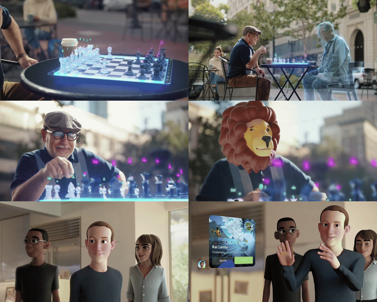
With the advent of devices like Meta Quest and Apple Vision Pro, Metaverse is gaining popularity among common people with human-like features, facial emotions, expressions, movements, etc. To create immersive experiences, we would need to witness realistic avatars of people who we communicate with from anywhere in the world. This is where Human Vision Models are game changers in creating life-like avatars.
Sapiens embodies the collective attributes of a good human-centric model that should have better generalization in varied conditions, broad applicability with minimal modifications and high fidelity to produce precise outputs.
Training Data Preparation for Sapiens
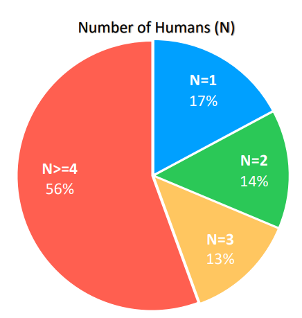
For pre-training in a self-supervised manner, the dataset used was a finely curated dataset with real and synthetic Humans-300M images in diverse conditions. There were 248 million images containing multiple human subjects.
Humans-300M is filtered from a large proprietary dataset of 1 billion human images excluding images with text, watermarks, artistic depictions, unnatural elements etc. Using bounding box detectors instances that have detection score of `0.9` and bounding box dimension more than 300 pixels were chosen. After pre-training, Sapiens was fine-tuned for individual tasks with specific datasets.
- Models were fine-tuned for pose-estimation,with dense set of 208 2D keypoints compassing body, feet,hands, surface and face.
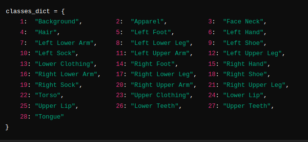
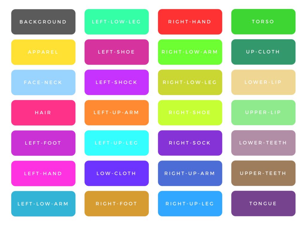
- Segmentation tasks were carried out on a detailed 28 classes vocabulary covering body parts such as hair, tongue, teeth, upper/lower hip and torso captured from multi-view to guarantee quality.
- Using platforms like Render People, detailed synthetic scans of depth maps and surface normal for 600 people are generated.
Model Variants

How was Sapiens Trained?
Sapiens natively supports 1024×1024 high-res images unlike previous SOTA models like Dino v2 which use 224×224. The Sapiens family of models are vision transformers built from scratch. They were first pre-trained using the Masked AutoEncoder (MAE) approach, followed by fine-tuning to a specific task. Pre-training was done using self-supervised training on an unlabelled Human-300M dataset with 1.2 trillion tokens. Similar to ViT, images are divided into non-overlapping fixed size patches.
Each image token (patch size = 16 x 16) is 0.02% of the entire image (1024×1024), unlike in a standard ViT a single patch accounts for 0.4%. This additional image tokens helps the model for better inter-token reasoning (between patches).
MASKED AUTO ENCODERS (MAE)
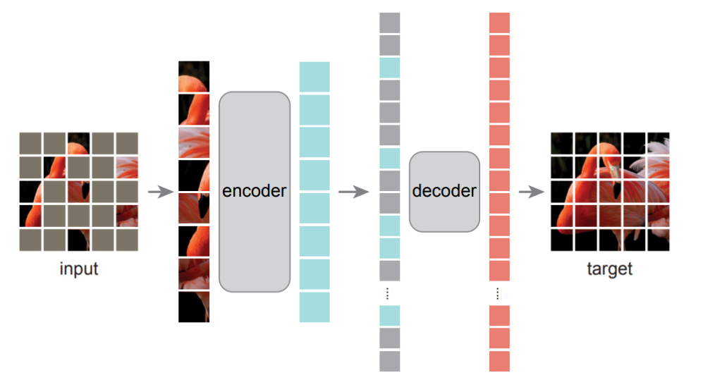
MAE processes a small subset of patches from the image, forcing the model to learn global features and approximately restore the missing patches. These sparse computations are aimed for efficient large-scale training by reducing the computational cost as fewer tokens are used. Like all autoencoders, the model has an encoder that maps only the visible patches from the masked images to latent representation. Then a decoder is used to reconstruct the missing patches pixel wise.
You may wonder if it doesn’t encode information about masked tokens then how the model is able to retain the spatial information. While the masked tokens aren’t encoded directly, the positional tokens of patches help to reconstruct the entire image. Typically MAE’s are trained with MSE Loss or reconstruction loss between the predicted and the original image pixels for the masked region.
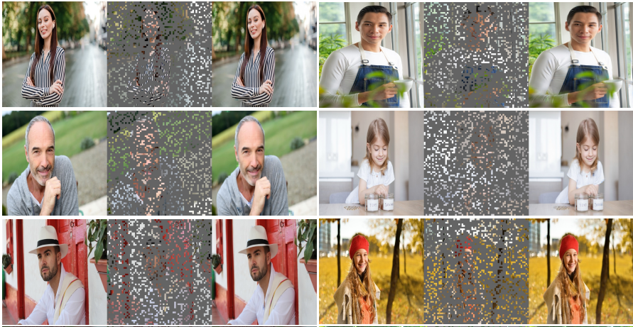
The following is the reconstruction results of Sapiens for varying mask ratio between 0.75 to 95%. Observe the last image in the grid with mask ratio of 95%, can you infer anything meaningful from the masked image? Nothing, right? Yet, we see that the model provides meaningful results even with 95% region masked in held out samples (test dataset). This highlights the model’s strong feature understanding about human subjects.

Task Specific Fine Tuning
Sapiens models are initialized with pre-trained weights for encoder and the decoder is a task-specific head initialized with random weights. During fine-tuning both the encoder and decoder are trained end-to-end.
1. 2D Pose Estimation

An input image of three channels along with bounding boxes is passed to the encoder as patches. The model follows a top-down approach, first the ROI (i.e. person) is detected and the keypoints are estimated for pose. Sapiens pose estimation model use heatmaps of each keypoint to determine the pose resulting K heatmaps for K keypoints.
Note: Each value in the Heatmap (2D matrix), represents the probability that a particular keypoint is at a specific spatial location.
![]()
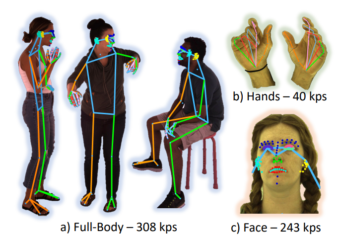
The training dataset contained 308 full-body key points where 243 particularly for facial keypoints and 40 hand key points while other pose estimation datasets usually have 68 facial keypoints. These helped in improved representation around eyes, lips, nose and ears.

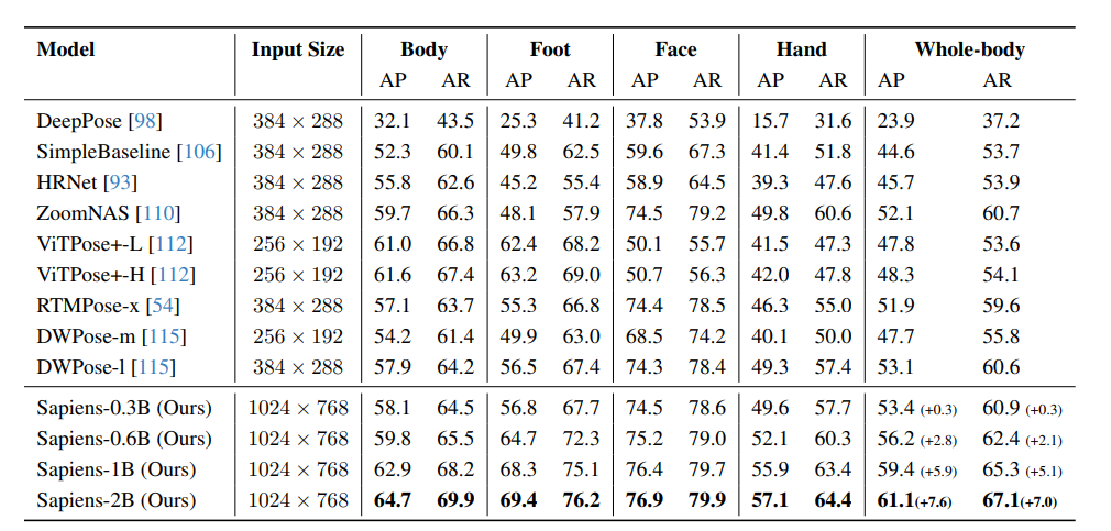
Metric Comparison
Sapiens 2B is the SOTA human pose estimation model achieving a highest AP on Humans-5K test dataset. It outperforms DWPose-L by +7.1 AP.
2.Body-Part Segmentation
The objective of this task is to classify each pixel in the input image (I) into C classes (Multi-class Segmentation) such as arm, leg, torso etc., For each pixel the model predicts a probability map that the pixel belongs to a particular class over all body parts. Weighted cross entropy loss was used in this task between predicted and ground truth parts segmentation masks.
![]()
The dataset used contains 0.1 M annotations that are manually created at 4k resolution. The model can predict 28 different body parts and it outlines finer details of limbs, legs, lips etc.

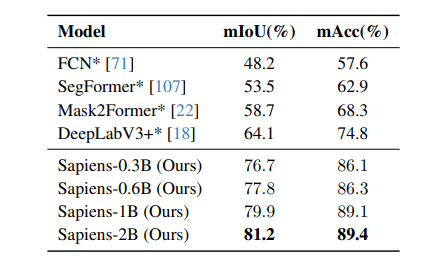
Metric Comparison
To evaluate performance on body-part segmentation tasks, models such as FCN, SegFormer, Mask2Former and DeepLabV3+ were fine-tuned and tested on the same dataset used for training Sapiens. As expected, the smallest Sapiens 0.3B model, outperformed previous SOTA models like Mask2Former and DeepLabV3+. The largest model Sapiens-2B achieves an outstanding performance with an 81.2 mIOU and 89.4 mAcc on the Humans-2K test set.
3. Depth Estimation
The depth estimation architecture is similar to segmentation, but the decoder’s output channel is modified to 1. Because depth estimation is a regression task, where output is a single depth value for each pixel rather than multi-class probability maps. To calculate relative depth, the depth value is normalized between 0 and 1 using maximum and minimum pixel value.
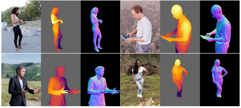
For effective training 0.5M synthetic images from 600 high-res human scans are used. A virtual camera is positioned within the scene and focal length, translation, rotation and camera is calibrated to obtain diverse depth maps at 4K resolution.
![]()
Metric Comparison

Dataset like TFHuman2.0 and Hi4D which contain single human scans and multi-human scenarios were used for reporting the RMSE metrics (lower is better) of Sapiens against MiDAS and DepthAnything. From the table we can infer that in most cases, all variants of Sapiens clearly perform better than their counterparts.

4. Surface Normal Estimation
A surface normal of a human body is a vector that is perpendicular to the surface at a given point in the body. It refers to the orientation of the surface in a 3D space.
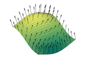
Source Wiki
Surface normals are particularly helpful in determining how the light interacts with the body’s surface to create realistic reflections.
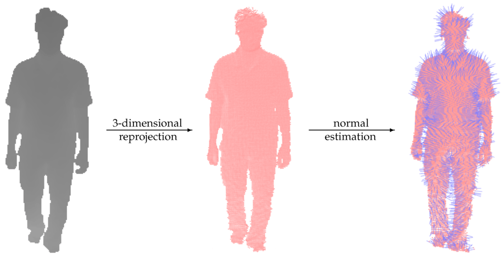
Source httpswwwmdpicom1424 8220194891
In Sapiens model, the surface normal estimator N generates 3 output channels corresponding to the normal’s x,y,z coordinates for each pixel of a human image. It refers to the orientation of the surface in 3D space.
![]()
where, ![]() is L1 Norm between ground truth and predicted normal,
is L1 Norm between ground truth and predicted normal,
![]() is a measure of how predicted normal orientation w.r.t ground truth normal.
is a measure of how predicted normal orientation w.r.t ground truth normal.
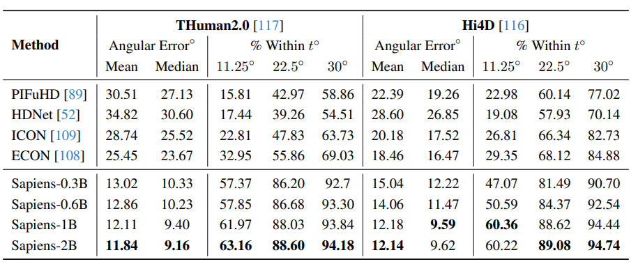
Metric Comparison
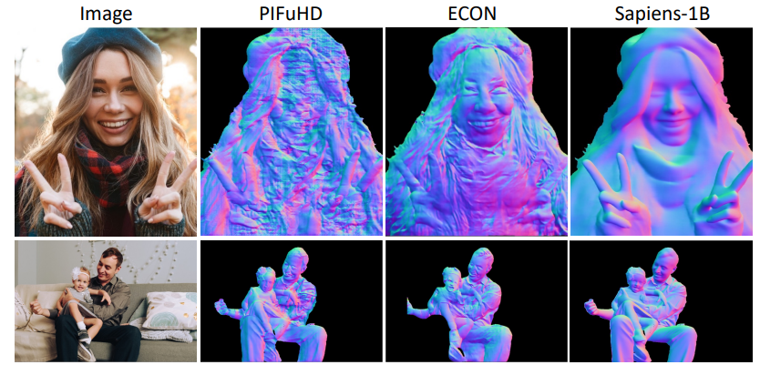
Same datasets from depth estimation are used for evaluating models performance on similar surface normal estimation tasks. Here also we observe Sapiens-2B consistently archives a very low mean angular error of 11.84.
Experimental Details of Sapiens
All the experiments were conducted using AdamW with learning rate schedulers that include linear warm up followed by cosine annealing. Standard augmentations like cropping, scaling, flipping and photometric distortions were applied. All the models were pre trained with an image size of 1024×1024 and a patch size = 16. During fine-tuning the input images were maintained at an aspect ratio of 4:3 (i.e. 1024×768).
Code Walkthrough
Disclaimer
All the results we are about to show were inferred using the gradio app of Sapiens official HuggingFace Spaces . However, to get some hands-on experience, we will go through some code sections to better understand how the preprocessing, model inference and post processing are done for each task.
Also to note that, with Huggingface spaces, you only get limited GPU quota. Therefore you can run the Sapiens gradio app demos locally, by simply cloning the task specific HuggingFace repositories.
We will make use of a simple Sapiens inference pipeline, which helps us get rid of additional complexities.
!git clone https://github.com/ibaiGorordo/Sapiens-Pytorch-Inference.git
%cd Sapiens-Pytorch-Inference
!pip install -r requirements.txt -q
import os
import sys
import shutil
from typing import List
import requests
from tqdm import tqdm
from datetime import timedelta

from enum import Enum
import time
import cv2
import numpy as np
import matplotlib.pyplot as plt
from imread_from_url import imread_from_url

from dataclasses import dataclass
from torchvision import transforms
import torch
import torch.nn.functional as F

from huggingface_hub import hf_hub_download, hf_hub_url
Download assets
import os
os.makedirs("test_images/", exist_ok = True)

!wget -nc https://learnopencv.com/wp-content/uploads/2024/09/man-horse-arrow-scaled.jpg -O test_images/man-horse-arrow.jpg

!wget -nc https://learnopencv.com/wp-content/uploads/2024/09/football-soccer-scaled.jpg -O test_images/football.jpg
!wget -nc https://learnopencv.com/wp-content/uploads/2024/09/jogging-1-scaled.jpg -O test_images/jogging.jpg

!wget -nc https://learnopencv.com/wp-content/uploads/2024/09/Sapiens-video-test.mp4 -O test_images/Sapiens-video-test.mp4
Download model checkpoints
We will choose, Sapiens-1B model for all of the upcoming sections, as it performs consistently across all types of tasks. Also we can fit the 1B model in Colab T4 by taking performance v/s resource factor into consideration.
Let’s download their checkpoints in torch script format from hugging face.
!wget -nc https://huggingface.co/facebook/sapiens-normal-1b-torchscript/resolve/main/sapiens_1b_normal_render_people_epoch_115_torchscript.pt2  -O models/sapiens_1b_normal_render_people_epoch_115_torchscript.pt2

!wget -nc https://huggingface.co/facebook/sapiens-seg-1b-torchscript/resolve/main/sapiens_1b_goliath_best_goliath_mIoU_7994_epoch_151_torchscript.pt2 -O models/sapiens_1b_goliath_best_goliath_mIoU_7994_epoch_151_torchscript.pt2

!wget -nc https://huggingface.co/facebook/sapiens-depth-1b-torchscript/resolve/main/sapiens_1b_render_people_epoch_88_torchscript.pt2 -O models/sapiens_1b_render_people_epoch_88_torchscript.pt2

!wget -nc https://huggingface.co/facebook/sapiens-pose-1b-torchscript/resolve/main/sapiens_1b_goliath_best_goliath_AP_640_torchscript.pt2 -O models/sapiens_1b_goliath_best_Sapiens-1B-Depth-Estimation-Single-Person-Inference-Results.jpggoliath_AP_640_torchscript.pt2
Common Utilities
To perform any type of task we will need some common helper functions, like downloading the model and preprocessing. We will be defining them below.
class TaskType(Enum):
    DEPTH = "depth"
    NORMAL = "normal"
    SEG = "seg"
    POSE = "pose"


def download(url: str, filename: str):
    with open(filename, "wb") as f:
        with requests.get(url, stream=True) as r:
            r.raise_for_status()
            total = int(r.headers.get("content-length", 0))

            # tqdm has many interesting parameters. Feel free to experiment!
            tqdm_params = {
                "total": total,
                "miniters": 1,
                "unit": "B",
                "unit_scale": True,
                "unit_divisor": 1024,
            }
            with tqdm(**tqdm_params) as pb:
                for chunk in r.iter_content(chunk_size=8192):
                    pb.update(len(chunk))
                    f.write(chunk)


def download_hf_model(model_name: str, task_type: TaskType, model_dir: str = "models"):
    if not os.path.exists(model_dir):
        os.makedirs(model_dir)

    path = model_dir + "/" + model_name
    if os.path.exists(path):
        return path

    print(f"Model {model_name} not found, downloading from Hugging Face Hub...")

    model_version = "_".join(model_name.split("_")[:2])
    repo_id = "facebook/sapiens"
    subdirectory = (
        f"sapiens_lite_host/torchscript/{task_type.value}/checkpoints/{model_version}"
    )

    # hf_hub_download(repo_id=repo_id, filename=model_name, subfolder=subdirectory, local_dir=model_dir)
    url = hf_hub_url(repo_id=repo_id, filename=model_name, subfolder=subdirectory)
    download(url, path)
    print("Model downloaded successfully to", path)

    return path
Basic preprocessing steps will be carried out using this create_preprocessor() function. It will take the input image and convert it to a PIL object. Then it resizes, normalizes and adds a batch dimension along axis=0.
def create_preprocessor(input_size: tuple[int, int],
                        mean: List[float] = (0.485, 0.456, 0.406),
                        std: List[float] = (0.229, 0.224, 0.225)):
    return transforms.Compose([transforms.ToPILImage(),
                               transforms.Resize(input_size),
                               transforms.ToTenspecificsor(),
                               transforms.Normalize(mean=mean, std=std),
                               transforms.Lambda(lambda x: x.unsqueeze(0))
                               ])
TASK 1: DEPTH ESTIMATION
A simple enum class, SapiensDepthType is defined with a pre-trained DEPTH_1B model with filename. As we know Enum helps to define a collection of constant values, and makes the code more structured. Therefore, we can simply call SapiensDepthType.DEPTH_1B for the model’s filename.
class SapiensDepthType(Enum):
    OFF = "off"
    DEPTH_1B = "sapiens_1b_render_people_epoch_88_torchscript.pt2"
The SapiensDepth class takes the necessary arguments like model type and dtype. In the constructor the model is loaded and is set in eval() mode.
class SapiensDepth:
    def __init__(
        self,
        type: SapiensDepthType = SapiensDepthType.DEPTH_1B,
        device: torch.device = torch.device(
            "cuda" if torch.cuda.is_available() else "cpu"
        ),
        dtype: torch.dtype = torch.float32,
    ):
        path = download_hf_model(type.value, TaskType.DEPTH)
        model = torch.jit.load(path)
        model = model.eval()
        self.model = model.to(device).to(dtype)
        self.device = device
        self.dtype = dtype
        self.preprocessor = create_preprocessor(input_size=(1024, 768))
When SapiensDepth() is called, the input image is preprocessed and is moved to a specified device ( cuda). To note that, the model expects the input to be in BGR format. By setting torch.inference_mode() the input is forward passed and the output results are further post processed using processor_depth() function to return the depth map.
 class SapiensDepth():
     . . . .
   def __call__(self, img: np.ndarray) -> np.ndarray:
        start = time.perf_counter()

        # Model expects BGR, but we change to RGB here because the preprocessor will switch the channels also
        input = cv2.cvtColor(img, cv2.COLOR_BGR2RGB)
        tensor = self.preprocessor(input).to(self.device).to(self.dtype)

        with torch.inference_mode():
            results = self.model(tensor)

        depth_map = postprocess_depth(results, img.shape[:2])
        print(f"Depth inference took: {time.perf_counter() - start:.4f} seconds")
        return depth_map
Once we get output results, we upsample it to the original image dimensions, convert it to a numpy array and remove its batch dimension.
def postprocess_depth(results: torch.Tensor, img_shape: tuple[int, int]) -> np.ndarray:
    result = results[0].cpu()

    # Upsample the result to the original image size
    logits = F.interpolate(
        result.unsqueeze(0), size=img_shape, mode="bilinear"
    ).squeeze(0)

    # Covert to numpy array
    depth_map = logits.float().numpy().squeeze()
    return depth_map
At last the draw_depth_map() takes in the numpy array of depth map and normalizes it based on min and max depth values of the overall image. This results in a normal distribution of pixel values in the range 0 to 1. By using OpenCV colormap utility, colors are assigned to each pixel which helps to differentiate contrast between nearest and farthest depth pixels. The brighter pixels represent closer instances and dark colors means distant ones. Any pixels apart from this is considered as background and is set to a pixel value of 128.
def draw_depth_map(depth_map: np.ndarray) -> np.ndarray:
    min_depth, max_depth = np.min(depth_map), np.max(depth_map)

    norm_depth_map = 1 - (depth_map - min_depth) / (max_depth - min_depth)
    norm_depth_map = (norm_depth_map * 255).astype(np.uint8)

    # Normalize and color the image
    color_depth = cv2.applyColorMap(norm_depth_map, cv2.COLORMAP_INFERNO)
    color_depth[depth_map == 0] = 128 #background
    return color_depth
Let’s execute this, all the above discussed functionalities to obtain the depth map. We will load the model weights in float16 precision in Colab’s T4. However if your GPU is of the latest architecture and supports bfloat16, it is recommended to use to use for better performance. To save the output in the original input dimension using matplotlib savefig(), make sure to use dpi=100.
To prevent OOM errors in Colab, we delete the model instance every time and empty the cuda cache. From our experimentation, we observe that for depth estimation tasks, nearly 7 GB vRAM was used.
if __name__ == "__main__":
    type = torch.float16
    device = torch.device("cuda" if torch.cuda.is_available() else "cpu")

    # Load the image
    img_path = "test_images/man-horse-bow-arrow.jpg"
    img = cv2.imread(img_path)

    # Initialize the depth estimator
    model_type = SapiensDepthType.DEPTH_1B
    estimator = SapiensDepth(model_type)

    # Estimate depth and measure time
    start = time.perf_counter()
    depth_map = estimator(img)  # Use the RGB image for depth estimation
    print(f"Time taken: {time.perf_counter() - start:.4f} seconds")

    # Draw the depth map
    depth_img = draw_depth_map(depth_map)

    # Convert depth_img from BGR to RGB for visualization and saving
    depth_img_rgb = cv2.cvtColor(depth_img, cv2.COLOR_BGR2RGB)

    height, width, _ = depth_img_rgb.shape

    fig = plt.figure(figsize = (width/100, height/100), dpi=100)

    # Display and save the RGB deSapiens-1B-Depth-Estimation-Single-Person-Inference-Results.jpgpth image
    plt.imshow(depth_img_rgb)
    plt.axis('off')  # Hide the axisspecific

    # Save the depth image as RGB
    plt.savefig("depth_image_rgb.png", bbox_inches='tight', pad_inches=0)
    plt.show()

    # Free the GPU memory
    del estimator  # Delete the model
    torch.cuda.empty_cache()  # Clear the GPU cache
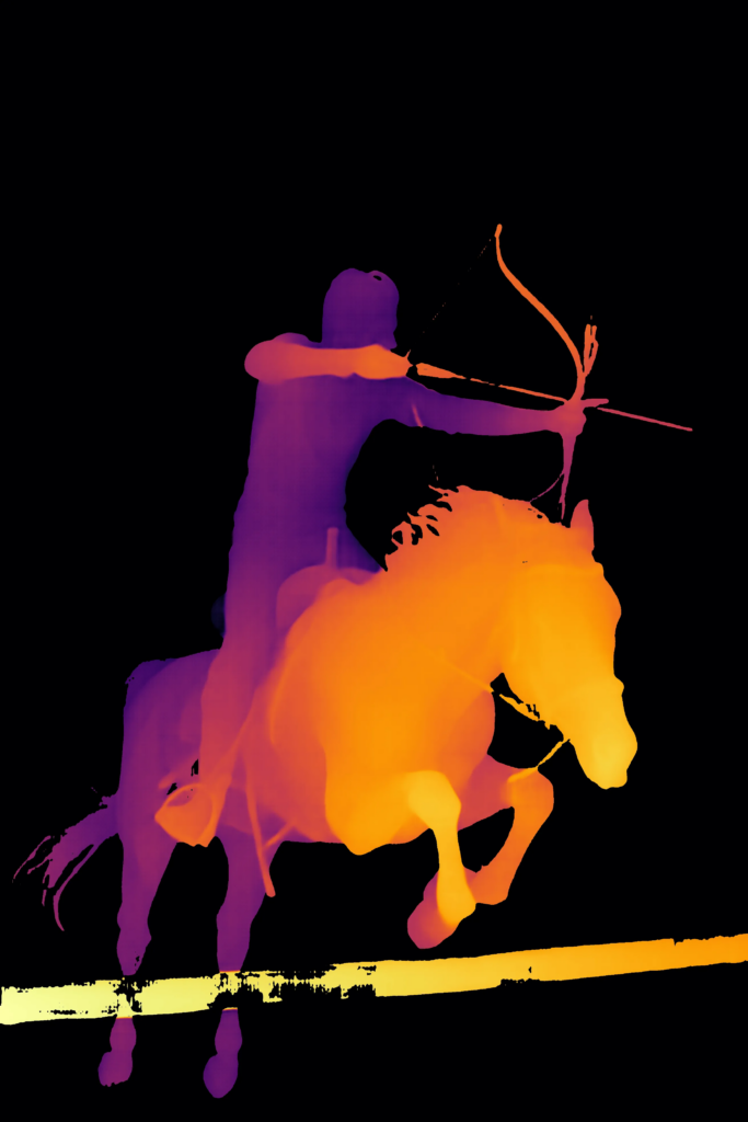
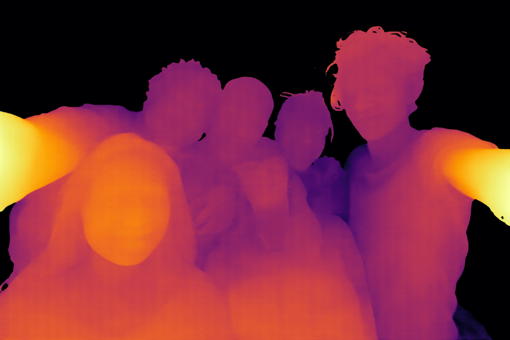
For depth estimation and surface normal prediction results we can observe that the model performs exceptionally well for non-human subjects as the author rightly discussed this in the paper.
Additionally, fb-bg-1b model is used to remove background before passing it to the Sapiens model (depth and surface normal) in HugingFace Space. In our code we aren’t utilizing the background removal model, owing to compute resource limitations.
Result 1: Single Person
Result 2: Multiple Person
TASK 2: SURFACE NORMAL ESTIMATION
Similar to Depth Estimation, SapiensNormal() is defined with some changes in draw_normal_map() and post processing steps.
class SapiensNormalType(Enum):
     OFF = "off"
     NORMAL_1B = "sapiens_1b_normal_render_people_epoch_115_torchscript.pt2"
class SapiensNormal:
    def __init__(
        self,
        type: SapiensNormalType = SapiensNormalType.NORMAL_1B,
        device: torch.device = torch.device(
            "cuda" if torch.cuda.is_available() else "cpu"
        ),
        dtype: torch.dtype = torch.float32,
    ):
        path = download_hf_model(type.value, TaskType.NORMAL)
        model = torch.jit.load(path)
        model = model.eval()
        self.model = model.to(device).to(dtype)
        self.device = device
        self.dtype = dtype
        self.preprocessor = create_preprocessor(
            input_size=(1024, 768)
        )  # Only these values seem to work well

    def __call__(self, img: np.ndarray) -> np.ndarray:
        start = time.perf_counter()

        # Model expects BGR, but we change to RGB here because the preprocessor will switch the channels also
        input = cv2.cvtColor(img, cv2.COLOR_BGR2RGB)
        tensor = self.preprocessor(input).to(self.device).to(self.dtype)

        with torch.inference_mode():
            results = self.model(tensor)

        normals = postprocess_normal(results, img.shape[:2])
        print(f"Normal inference took: {time.perf_counter() - start:.4f} seconds")
        return normals
To be compatible with the post processing and visualization utilities, we will need to upsample with bilinear interpolation and rearrange the output normal map to have the channel dimension at last (height, width, channels).
def postprocess_normal(results: torch.Tensor, img_shape: tuple[int, int]) -> np.ndarray:
    result = results[0].detach().cpu()

    # Upsample the result to the original image size
    logits = F.interpolate(
        result.unsqueeze(0), size=img_shape, mode="bilinear"
    ).squeeze(0)

    # Covert to numpy array
    normal_map = logits.float().numpy().transpose(1, 2, 0)

    return normal_map
A normal map typically stores surface normals in a 3D space (x,y,z) with pixel values between -1 and 1. But OpenCV expects pixel values in the range of 0 to 255. So at first we will need to normalize between 0 to 1 using the norm unit vector (normal_map_norm). Then by multiplying 255, we scale the pixel values between 0 and 255.
def draw_normal_map(normal_map: np.ndarray) -> np.ndarray:

    # Normalize the normal map
    normal_map_norm = np.linalg.norm(normal_map, axis=-1, keepdims=True)
    normal_map_normalized = normal_map / (
        normal_map_norm + 1e-5
    )  # Add epsilon to avoid division by zero

    # Scale normalized values to [0, 255] range
    normal_map = ((normal_map_normalized + 1) / 2 * 255).astype(np.uint8)

    # Convert the normal map to BGR format
    return cv2.cvtColor(normal_map, cv2.COLOR_RGB2BGR)
In the similar manner before, we will combine all functionalities to obtain surface normal results.
if __name__ == "__main__":

    img_path = "test_images/man-horse-arrow.jpg"
    img = cv2.imread(img_path)

    model_type = SapiensNormalType.NORMAL_1B
    estimator = SapiensNormal(model_type)

    start = time.perf_counter()
    normals = estimator(img)
    print(f"Time taken: {time.perf_counter() - start:.4f} seconds")

    normal_img = draw_normal_map(normals)

    # Convert depth_img from BGR to RGB for visualization and saving
    normal_img_rgb = cv2.cvtColor(normal_img, cv2.COLOR_BGR2RGB)

    height, width, _ = normal_img_rgb.shape

    fig = plt.figure(figsize = (width/100, height/100), dpi=100)

    # Display and save the RGB depth image
    plt.imshow(normal_img_rgb)
    plt.axis('off')  # Hide the axis

    # Save the depth image as RGB
    plt.savefig("normal_image_rgb.png", bbox_inches='tight', pad_inches=0)
    plt.show()

    # Free the GPU memory
    del estimator  # Delete the model
    torch.cuda.empty_cache()  # Clear the GPU cache
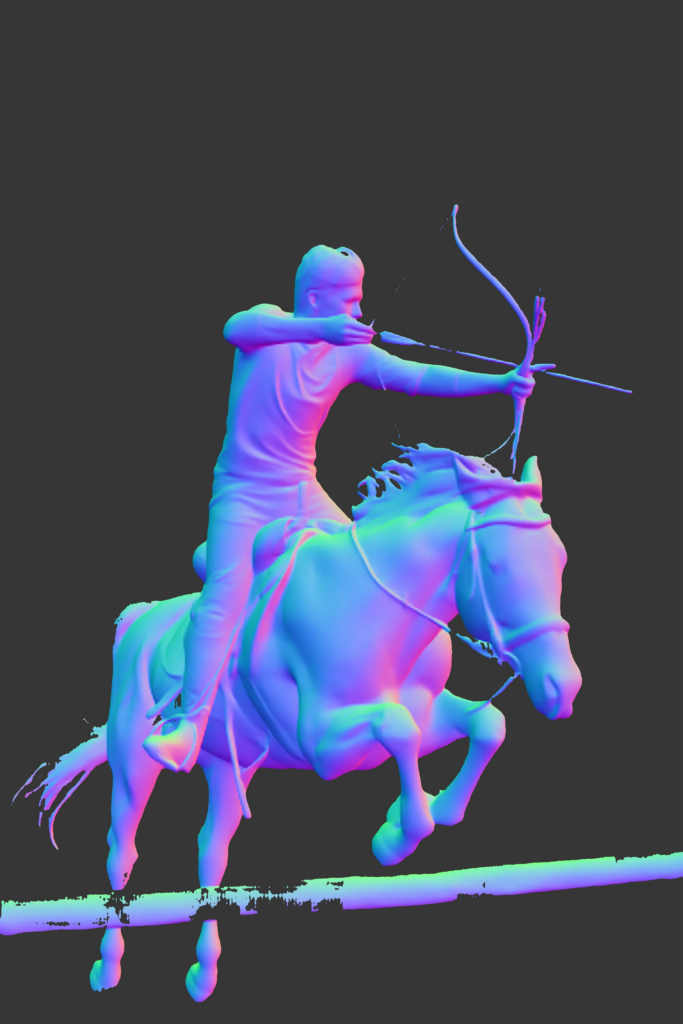
Result 1: Single Person
Result 2: Multiple Person
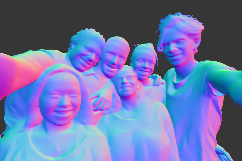
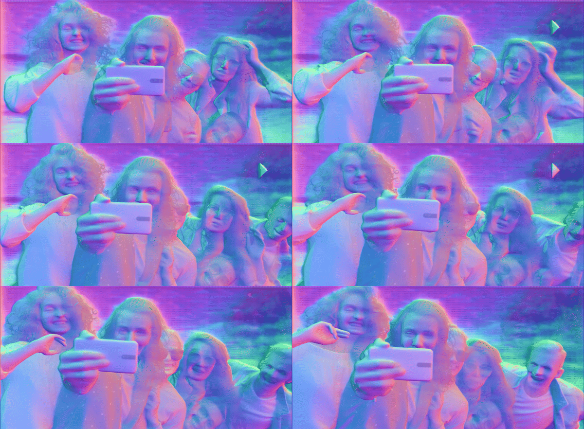
TASK 3: BODY PART-SEGMENTATION
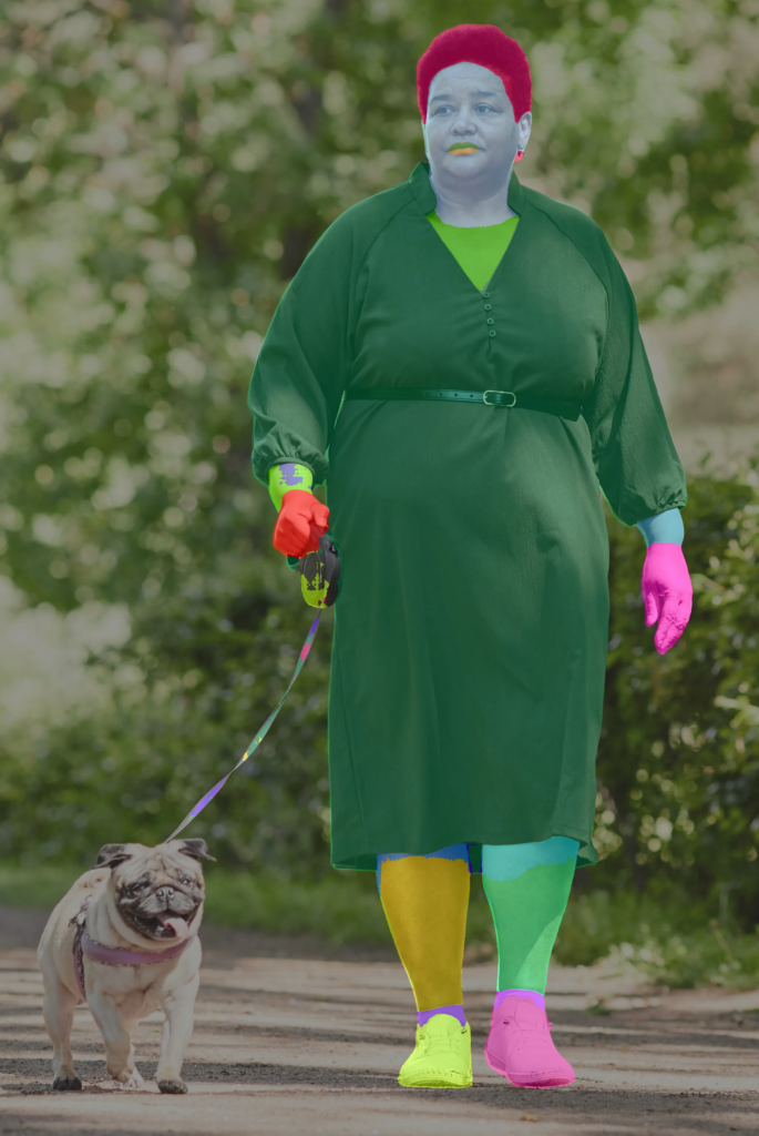
Sapiens model can detect 28 different human body parts, we can get the same colormap for each class, as mentioned in the paper by using a seed value of 11 in randint() for reproducibility.
class SapiensSegmentationType(Enum):
    SEGMENTATION_1B = (
        "sapiens_1b_goliath_best_goliath_mIoU_7994_epoch_151_torchscript.pt2"
    )


random = np.random.RandomState(11)

# --------------------------------**** 28 Classes **** -------------------------------------------------

classes = [
    "Background",
    "Apparel",
    "Face Neck",
    "Hair",
    "Left Foot",
    "Left Hand",
    "Left Lower Arm",
    "Left Lower Leg",
    "Left Shoe",
    "Left Sock",
    "Left Upper Arm",
    "Left Upper Leg",
    "Lower Clothing",
    "Right Foot",
    "Right Hand",
    "Right Lower Arm",
    "Right Lower Leg",
    "Right Shoe",
    "Right Sock",
    "Right Upper Arm",
    "Right Upper Leg",
    "Torso",
    "Upper Clothing",
    "Lower Lip",
    "Upper Lip",
    "Lower Teeth",
    "Upper Teeth",
    "Tongue",
]

colors = random.randint(0, 255, (len(classes) - 1, 3))
colors = np.vstack((np.array([128, 128, 128]), colors)).astype(
    np.uint8
)  # Add background color
colors = colors[:, ::-1]
class SapiensSegmentation:
    def __init__(
        self,
        type: SapiensSegmentationType = SapiensSegmentationType.SEGMENTATION_1B,
        device: torch.device = torch.device(
            "cuda" if torch.cuda.is_available() else "cpu"
        ),
        dtype: torch.dtype = torch.float32,
    ):
        path = download_hf_model(type.value, TaskType.SEG)
        model = torch.jit.load(path)
        model = model.eval()
        self.model = model.to(device).to(dtype)
        self.device = device
        self.dtype = dtype
        self.preprocessor = create_preprocessor(
            input_size=(1024, 768)
        )  # Only these values seem to work well

    def __call__(self, img: np.ndarray) -> np.ndarray:
        start = time.perf_counter()

        # Model expects BGR, but we change to RGB here because the preprocessor will switch the channels also
        input = cv2.cvtColor(img, cv2.COLOR_BGR2RGB)
        tensor = self.preprocessor(input).to(self.device).to(self.dtype)

        with torch.inference_mode():
            results = self.model(tensor)
        segmentation_map = postprocess_segmentation(results, img.shape[:2])

        print(f"Segmentation inference took: {time.perf_counter() - start:.4f} seconds")
        return segmentation_map
Just like usual segmentation tasks, the single channel mask (segmentation map) is expanded to 3-channel image, and each pixel value is assigned a pred-defined color corresponding to its class.
def draw_segmentation_map(segmentation_map: np.ndarray) -> np.ndarray:
    h, w = segmentation_map.shape #single channel
    segmentation_img = np.zeros((h, w, 3), dtype=np.uint8) #3 channels

    for i, color in enumerate(colors):
        segmentation_img[segmentation_map == i] = color

    return segmentation_img
For a multi-class segmentation, the model outputs a tensor with shape (num_classes, height, width). By taking argmax, the index of class whichever has the highest probability of is returned. By this we generate our final body-part segmentation map. For a proper visualization, we will use cv2.addWeighted() to blend the mask on top of the original image.
def postprocess_segmentation(results: torch.Tensor, img_shape: tuple[int, int]) -> np.ndarray:
    result = results[0].cpu()

    # Upsample the result to the original image size
    logits = F.interpolate(result.unsqueeze(0), size=img_shape, mode="bilinear").squeeze(0)

    # Perform argmax to get the segmentation map
    segmentation_map = logits.argmax(dim=0, keepdim=True)

    # Covert to numpy array
    segmentation_map = segmentation_map.float().numpy().squeeze()

    return segmentation_map
if __name__ == "__main__":

    img_path = "test_images/man-horse-arrow.jpg"
    img = cv2.imread(img_path)

    model_type = SapiensNormalType.NORMAL_1B
    estimator = SapiensNormal(model_type)

    start = time.perf_counter()
    normals = estimator(img)
    print(f"Time taken: {time.perf_counter() - start:.4f} seconds")

    normal_img = draw_normal_map(normals)

    # Convert depth_img from BGR to RGB for visualization and saving
    normal_img_rgb = cv2.cvtColor(normal_img, cv2.COLOR_BGR2RGB)

    height, width, _ = normal_img_rgb.shape

    fig = plt.figure(figsize = (width/100, height/100), dpi=100)

    # Display and save the RGB depth image
    plt.imshow(normal_img_rgb)
    plt.axis('off')  # Hide the axis

    # Save the depth image as RGB
    plt.savefig("normal_image_rgb.png", bbox_inches='tight', pad_inches=0)
    plt.show()

    # Free the GPU memory
    del estimator  # Delete the model
    torch.cuda.empty_cache()  # Clear the GPU cache
To get intuition about different part segmentation shown in the result section, we can mind map the color from the following palette.
Result 1: Single Person
Result 2: Multiple Person
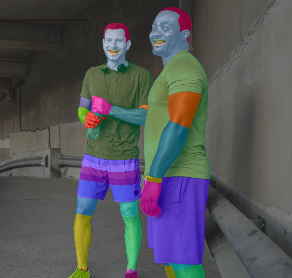
TASK 4: POSE ESTIMATION
As we discussed in an earlier section, before passing to the pose estimator model, we will use any object detector to crop the human subject. In official hugging face repo authors, use rtmdet_m_8xb32 model which requires to set up mmlab. However to keep things simple, we will use the yolov8m model from ultralytics as the detector. This will return the bboxes of human instances detected.
from ultralytics import YOLO


@dataclass
class DetectorConfig:
    model_path: str = "models/yolov8m.pt"
    person_id: int = 0
    conf_thres: float = 0.25


def draw_boxes(img, boxes, color=(0, 255, 0), thickness=2):
    draw_img = img.copy()
    for box in boxes:
        x1, y1, x2, y2 = box
        draw_img = cv2.rectangle(draw_img, (x1, y1), (x2, y2), color, thickness)
    return draw_img


class Detector:
    def __init__(self, config: DetectorConfig = DetectorConfig()):
        model_path = config.model_path
        if not model_path.endswith(".pt"):
            model_path = model_path.split(".")[0] + ".pt"
        self.model = YOLO(model_path)
        self.person_id = config.person_id
        self.conf_thres = config.conf_thres

    def __call__(self, img: np.ndarray) -> np.ndarray:
        return self.detect(img)

    def detect(self, img: np.ndarray) -> np.ndarray:
        start = time.perf_counter()
        results = self.model(img, conf=self.conf_thres)
        detections = results[0].boxes.data.cpu().numpy()  # (x1, y1, x2, y2, conf, cls)

        # Filter out only person
        person_detections = detections[detections[:, -1] == self.person_id]
        boxes = person_detections[:, :-2].astype(int)

        print(f"Detection inference took: {time.perf_counter() - start:.4f} seconds")
        return boxes
From Hugging Face, we will download the pose visualization utility from hugging face. This script file contains a dictionary of keypoint names (named as GOLIATH_KEYPOINTS), color maps for each keypoints.
!wget https://huggingface.co/spaces/facebook/sapiens-pose/resolve/main/classes_and_palettes.py -O classes_and_palettes.py
from classes_and_palettes import (
    COCO_KPTS_COLORS,
    COCO_WHOLEBODY_KPTS_COLORS,
    GOLIATH_KPTS_COLORS,
    GOLIATH_SKELETON_INFO,
    GOLIATH_KEYPOINTS,
)


class SapiensPoseEstimationType(Enum):
    POSE_ESTIMATION_1B = "sapiens_1b_goliath_best_goliath_AP_640_torchscript.pt2"
As usual, the SapiensPoseEstimation class comprises detector, preprocessor, model loading etc., within its constructor.
class SapiensPoseEstimation:
    def __init__(
        self,
        type: SapiensPosestimationType = SapiensPoseEstimationType.POSE_ESTIMATION_1B,
        device: torch.device = torch.device(
            "cuda" if torch.cuda.is_available() else "cpu"
        ),
        dtype: torch.dtype = torch.float32,
    ):
        # Load the model
        self.device = device
        self.dtype = dtype
        path = download_hf_model(type.value, TaskType.POSE)
        self.model = torch.jit.load(path).eval().to(device).to(dtype)
        self.preprocessor = create_preprocessor(input_size=(1024, 768))
        # Initialize the YOLO-based detector
        self.detector = Detector()
Then, we instantiate the pose estimation model as estimate_pose which takes in the input image and the boxes returned from the detector model. From this we obtain a set of 308 body keypoints.
class SapiensPoseEstimation:
     . . . .

   def __call__(self, img: np.ndarray) -> np.ndarray:
        start = time.perf_counter()

        # Detect persons in the image
        bboxes = self.detector.detect(img)

        # Process the image and estimate the pose
        pose_result_image, keypoints = self.estimate_pose(img, bboxes)

        print(f"Pose estimation inference took: {time.perf_counter() - start:.4f} seconds")
        return pose_result_image, keypoints
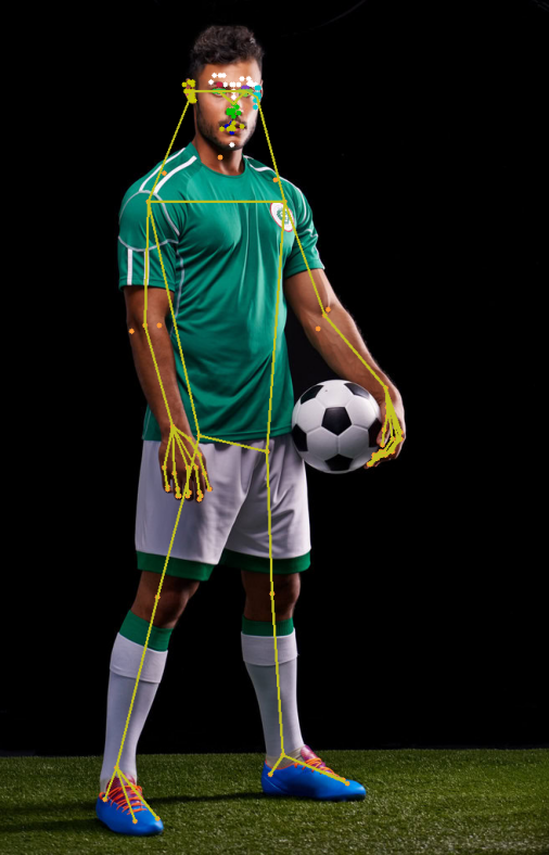
The GOLIATH pose estimation model returns, heatmap tensors of shape (num_heatmaps, height, width). Each heatmap shows how likely a certain keypoint is located at a pixel position. Then function np.argmax(heatmaps[i]) returns the most likely position of a keypoint based on the maximum value in the heatmap. Followed by this, np.unravel_index() converts heatmap into 2D coordinates(x,y) location of all key points within the heatmap. Finally we return key points of shape (x,y,confidence).
class SapiensPoseEstimation:
     . . . .
    def heatmaps_to_keypoints(self, heatmaps: np.ndarray) -> dict:
        keypoints = {}
        for i, name in enumerate(GOLIATH_KEYPOINTS):
            if i < heatmaps.shape[0]:
                y, x = np.unravel_index(np.argmax(heatmaps[i]), heatmaps[i].shape)
                conf = heatmaps[i, y, x]
                keypoints[name] = (float(x), float(y), float(conf))
        return keypoints
class SapiensPoseEstimation:
    . . . .
    @torch.inference_mode()
    def estimate_pose(
        self, img: np.ndarray, bboxes: List[List[float]]
    ) -> (np.ndarray, List[dict]):
        all_keypoints = []
        result_img = img.copy()

        for bbox in bboxes:
            cropped_img = self.crop_image(img, bbox)
            tensor = (
                self.preprocessor(cropped_img)
                .unsqueeze(0)
                .to(self.device)
                .to(self.dtype)
            )

            heatmaps = self.model(tensor)
            keypoints = self.heatmaps_to_keypoints(heatmaps[0].cpu().numpy())
            all_keypoints.append(keypoints)

            # Draw the keypoints on the original image
            result_img = self.draw_keypoints(result_img, keypoints, bbox)

        return result_img, all_keypoints

    def crop_image(self, img: np.ndarray, bbox: List[float]) -> np.ndarray:
        x1, y1, x2, y2 = map(int, bbox[:4])
        return img[y1:y2, x1:x2]
By using a simple utility function we draw keypoint based on the coordinates of locations returned after post processing.
class SapiensPoseEstimation:
     . . . .
    def draw_keypoints(
        self, img: np.ndarray, keypoints: dict, bbox: List[float]
    ) -> np.ndarray:
        x1, y1, x2, y2 = map(int, bbox[:4])
        bbox_width, bbox_height = x2 - x1, y2 - y1
        img_copy = img.copy()

        # Draw keypoints on the image
        for i, (name, (x, y, conf)) in enumerate(keypoints.items()):
            if conf > 0.3:  # Only draw confident keypoints
                x_coord = int(x * bbox_width / 192) + x1
                y_coord = int(y * bbox_height / 256) + y1
                cv2.circle(img_copy, (x_coord, y_coord), 3, GOLIATH_KPTS_COLORS[i], -1)

        # Optionally draw skeleton
        for _, link_info in GOLIATH_SKELETON_INFO.items():
            pt1_name, pt2_name = link_info["link"]
            if pt1_name in keypoints and pt2_name in keypoints:
                pt1 = keypoints[pt1_name]
                pt2 = keypoints[pt2_name]
                if pt1[2] > 0.3 and pt2[2] > 0.3:
                    x1_coord = int(pt1[0] * bbox_width / 192) + x1
                    y1_coord = int(pt1[1] * bbox_height / 256) + y1
                    x2_coord = int(pt2[0] * bbox_width / 192) + x1
                    y2_coord = int(pt2[1] * bbox_height / 256) + y1
                    cv2.line(
                        img_copy,
                        (x1_coord, y1_coord),
                        (x2_coord, y2_coord),
                        GOLIATH_KPTS_COLORS[i],
                        2,
                    )

        return img_copy
Result 1: Single Person
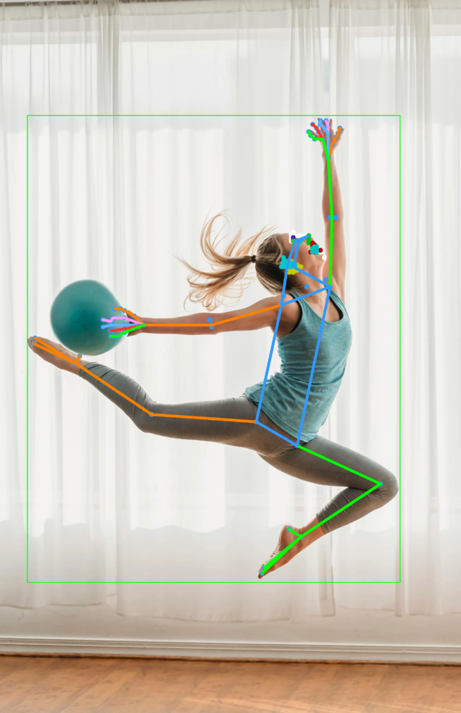
Result 2: Multiple Person
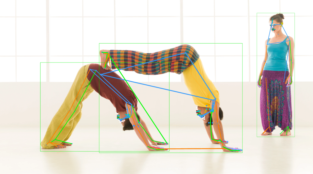
We see the model struggle in multiple person pose estimation , differentiating the lower part of the body in a slightly complex scene like this,
Key Takeaways
- By combining domain-specific large scale pretraining with high quality annotations, Sapiens models are robust to the four fundamental human-centric tasks at reduced computational complexity.
- While Sapiens perform well, they are not perfect and are still limited to complex poses, occlusion and crowded scenes.
Conclusion
We observed impressive predictions by the Sapiens-1B model across the four tasks. Despite some limitations, human centric models like Sapiens with their unified architecture are invaluable for creating realistic 3D avatars capable of handling multiple tasks with high precision. As mixed reality space is evolving we can expect to see more unified models like these playing critical roles for immersive metaverse experiences.
References
- Spl thanks to Ibai Goroda – for Sapiens inference pipeline
- Sapiens: Foundation for Human Vision Models
- Masked Autoencoders Are Scalable Vision Learners
- Sapiens Repository
- Session by Support Vectors on Sapiens
- AI Papers Academy






100K+ Learners
Join Free OpenCV Bootcamp3 Hours of Learning