In this post, we will discuss an object detection approach that leverages the understanding of the objects’ structure and the context of the image by enumerating objects’ characteristics and relations.
Such methods in computer vision are reminiscent of how humans recognize objects. They provide many advantages over other approaches for solving real-life problems.
After a short description of the problem, I will present a system I am developing that implements this approach. We will discuss many practical examples. I am also sharing links to my code in this post so you can modify it and try out the approach for yourself.
How Multiple Attributes Help in Object Detection
When a person wants to describe an object to another person, they usually name a set of characteristics or attributes. These attributes typically include shape, color, texture, size, material, and the presence of additional elements.
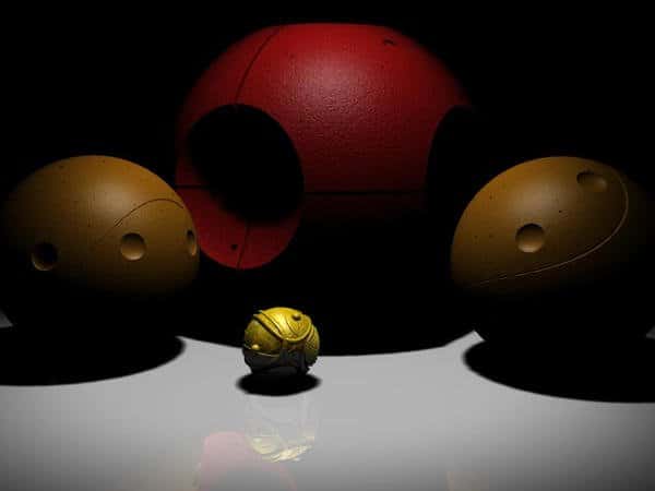
Let’s say you have not heard about the game of Quidditch in the Harry Potter series. We can describe a snitch as a small golden ball with retractable wings. This description will be enough to uniquely identify the snitch in the picture below.
Quidditch balls from the Harry Potter universe. They are not familiar to everyone, but the human ability to describe objects by recounting their attributes helps anyone select the correct one (image credit: deviantArt).
This natural method of describing an object via attributes is also used in computer vision [1]. There are different approaches to describing the attributes of an object: from classical to learned [2]. It helps generalize information about objects more qualitatively and improves recognition accuracy [3, 4]. It even enables the recognition of objects the system has not seen before [5, 6].
Another task is human-machine interaction [7]. I believe that the future of collaborative robots is not far off, and very soon, they will be as common in our homes as robotic vacuum cleaners. Unfortunately, like a person, a robot cannot know all possible objects in the environment. Therefore, it needs to describe an object as a set of attributes. Also, instances of the same object type can be present in the environment. For example, a picture may have a rack of shirts that look very different from each other. If we want to instruct the robot to “iron a shirt with a red stripe,” it must choose the correct one from all the found shirts.
All of them are shirts, but are they the same? (image credit: closetfactory)
So if the system can recognize shirts and classify different textures, it will be able to solve the problem by combining these attributes.
However, sometimes even this approach may not be enough for an accurate description. People often use contextual information from the environment of the described object. For example, when my father taught me to drive, he did not say that the gas pedal was the largest one. Instead, he said the gas pedal was on the right, the brake was in the middle, and the clutch was on the left.
Clutch and brake pedals look the same, but using spatial information, people can separate them from each other (image credit: mynrma).
This information is meaningless if you do not see all the pedals together. Objects connected by relationships are usually called a scene [8].
As you can see from the example, such a description allows you to significantly expand the information about objects and distinguish outwardly identical objects.
Graphs based methods for Object Detection
Working with scenes [9] is an attractive approach for many researchers in computer vision, especially since graphs can be used as a rigorous description of the scene, where the vertices of the graph are objects, and the edges are relations between objects [10].
The relations in the scenes can take different forms
- spatial (in front, to the right, above, inside);
- comparative (bigger, same, smaller);
- part-whole (to have/include, to be a part of);
- or have other specific semantics (hold, ride on, play on).
Also, graphs are attractive because we represent them as a matrix of connections between objects in deep machine learning methods. In [11], the authors present a good review of graph neural networks.
Proposed solution
System description
The approach of multiattribute and graph detection is also interesting from the point of view of a system for rapid prototyping of object recognition, which will allow combining existing developments in the field of computer vision within one architecture. This system has several advantages:
- it enables reusing already created methods of computer vision;
- it provides a simple toolkit for users who are not specialists in the field of computer vision;
- it allows solving problems for which the standard learning approach is challenging.
I could not find existing systems that would provide such functionality, so I decided to create my own. I called the system under development Extended Object Detection and only later found out about a module with this name in OpenCV.
My system has the following set of core entities:
- object attributes represented by the corresponding software detectors;
- simple objects, represented by a set of object attributes;
- relations between objects defined by the corresponding software detectors;
- complex objects, represented by a graph in which the vertices are simple objects, and the edges are relations.
Main entities of the proposed solution and their connections
The core of the system, like most attribute detectors, is written using OpenCV. However, the class abstraction allows you to integrate other C++ libraries. For example, we successfully integrated TensorFlow, Dlib, Zbar, and igraph.
Simple Object detection: Combining Multiple Attributes
Modern vision techniques can identify many attributes.
A neural network recognition is good at generalizing the idea of an object and acts as an attribute of a concept. Color filtering lets you add a color attribute that people regularly use to describe objects. Feature-based detection allows you to define the desired patterns in images, acting as texture attributes. Contour analysis methods will enable you to determine patterns in the shape of an object. Even a simple analysis of the bounding box will let you get some idea about the shape of an object and its dimensions. Each attribute highlights a different set of bounding boxes in the image.
Further, the system’s task is to highlight the areas in which all the attributes were positive. This process occurs iteratively. The first step is to combine the first attribute’s bounding boxes with the second attribute’s bounding boxes. We choose the IoU metric (ratio of intersection of boxes to the union of boxes) as a criterion for maximum likelihood estimation. A pair of bounding boxes with the maximum similarity is combined and removed from consideration. Then the procedure is repeated for the rest of the bounding boxes until they run out or there are no pairs with IoU values below the specified threshold. The combined result of the first and second attributes are similarly combined with the output of the third attribute and so on.
Attributes can be of three types:
- Detect – directly defining new areas in the image;
- Check – checking whether the already selected areas are satisfied with the specified parameters (size, pose, dimensions, etc.);
- Extract – Extraction of additional information, for example, orientation in space by a stereo camera.
Example 1. Select a specific cup from a set of other cups.
It is possible to train a classical neural network detector to recognize a specific cup, but not for all specific cups in the world. Neural networks instead learn a generalized understanding of what a cup is. So attribute description of an object allows using the neural network’s generalized understanding of the cup with the imposition of the required additional attributes.
The image below shows us cups of two different colors. I used a Convolutional Neural Network (CNN) based detector to detect two instances of cups. Then I applied an HSV color filtration technique to the original image to detect red spots on the image. Such techniques are pretty noisy and show five different results. Then both outputs were combined with the described method, and as a result, we got one red cup as desired.
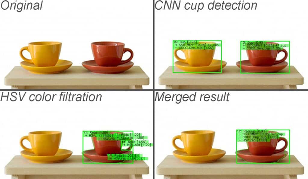
Using both CNN and color filtration techniques, we can detect the “red cup” object (source: freepik).
You can find the code for this recognition on Github. One of my desires was an abstraction from the API at the level of object description. So in most cases, you do not need to write the code. Instead, you can use an XML description of the objects and a general-purpose executable for object detection provided with the package. I wrote a simple application (dummy_console_app) that reads the XML file and performs detection on an input image.
I have also included a full list of applications at the end of this post. The file (I called it Object Base) that describes objects identical to the presented code is shown below:
<?xml version="1.0" ?>

<AttributeLib>

    <Attribute Name="HSV_red" Type="HSVColor" Hmin="0" Hmax="11" Smin="100" Smax="255" Vmin="10" Vmax="255"/>

    <Attribute Name="SSD_MNv1" Type="Dnn" framework="tensorflow" weights="ssd_mobilenet_v1_coco_2017_11_17/frozen_inference_graph.pb" config="ssd_mobilenet_v1_coco_2017_11_17/config.pbtxt" labels="ssd_mobilenet_v1_coco_2017_11_17/mscoco_label_map.pbtxt" inputWidth="300" inputHeight="300" Probability="0.1" forceCuda="0"/>

   <Attribute Name="COCO_Dnn_cup" Type="ExtractedInfoString" field="SSD_MNv1:class_label" allowed="cup" forbidden="" Weight="0"/>

</AttributeLib>

<SimpleObjectBase>

   <SimpleObject Name="Cup" ID="10">
        <Attribute Type="Detect">SSD_MNv1</Attribute>
        <Attribute Type="Check">COCO_Dnn_cup</Attribute>
    </SimpleObject>

   <SimpleObject Name="Reds" ID="11">
        <Attribute Type="Detect">HSV_red</Attribute>
    </SimpleObject>

   <SimpleObject Name="RedCup" ID="12" MergingPolicy="Union">
        <Attribute Type="Detect">SSD_MNv1</Attribute>
        <Attribute Type="Check">COCO_Dnn_cup</Attribute>
        <Attribute Type="Detect">HSV_red</Attribute>
    </SimpleObject>

</SimpleObjectBase>
The example shows three attributes – color filtering in the HSV space, a general neural network model, and an attribute of checking the label of the neural network output. Further, these attributes in various combinations are collected into simple objects. The recognition results for each object were presented in the figure above. A simple solution that reads the Object Base file, image, and the desired object to detect is available on Github.
Complex Objects detection : Using Multiple Attributes & Graphs
The previous example illustrated the recognition of the so-called simple object which is represented by a list of attributes. This description is not always sufficient to recognize the original object.
A complex object, represented in the form of a graph, consists of simple objects which are connected by relations. First, the system detects the entire set of simple objects, represented by bounding boxes, and creates an observation graph, adding all these objects as vertices. Next, the system checks pairwise simple objects for satisfaction with the given relations, and if the relation is satisfied, then connects the corresponding pair of vertices with an edge. After that, when the observation graph is formed, we need to find the complex object in it. To do that, the graph of the complex object must be mapped to the vertices and edges of the observation graph. Fortunately, this problem is well known and solved in graph theory by searching for an isomorphic subgraph. I use the igraph library implementation of the VF2 method for this. When relations between objects are not commutative, directed graphs are used.
Example 2. As a simple example, let’s try to recognize a person on a motorcycle using this system. In many popular object detectors, “person” and “motorcycle” objects are recognized separately. Let us combine these two objects with a “mount” relation. As mentioned above, we can also learn such relations from annotated data in the general case.
However, it can also be constructed from relatively simple geometric relationships that are implemented in the system. First, the center of the “person” object must be higher than the center of the “motorcycle” object. The objects must also have a non-zero intersection.
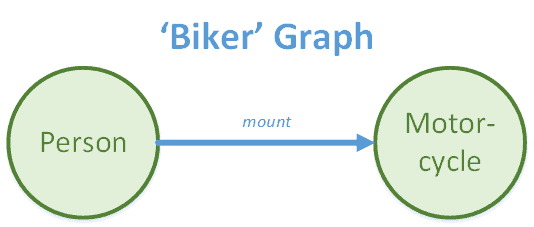
At this stage, I have not yet implemented a relation that checks two objects for the intersection of their bounding boxes. But I was able to implement it using existing relationships “inside” and “outside” and logical pseudo-relationships (AND, OR, NOT). So “intersects” is ((NOT “inside”) AND (NOT “outside”)). And the relation “mount” itself then takes the form (“up” AND “intersects”). The graph of this object looks trivial: two objects connected by a relation.
Graph representation of a ’Biker’ Complex Object which consists of a ‘person’ who ‘mounts’ a ‘motorcycle’
In the form of an XML-file Object Base, this object, as well as its constituent parts, are described as follows:
<?xml version="1.0" ?>

<AttributeLib>

    <Attribute Name="FRCNN_RN50" Type="Dnn" framework="tensorflow" weights="faster_rcnn_resnet50_coco_2018_01_28/frozen_inference_graph.pb" config="faster_rcnn_resnet50_coco_2018_01_28/config.pbtxt" labels="faster_rcnn_resnet50_coco_2018_01_28/mscoco_label_map.pbtxt" inputWidth="300" inputHeight="300" Probability="0.1" forceCuda="0"/>

    <Attribute Name="SSD_MNv1" Type="Dnn" framework="tensorflow" weights="ssd_mobilenet_v1_coco_2017_11_17/frozen_inference_graph.pb" config="ssd_mobilenet_v1_coco_2017_11_17/config.pbtxt" labels="ssd_mobilenet_v1_coco_2017_11_17/mscoco_label_map.pbtxt" inputWidth="300" inputHeight="300" Probability="0.1" forceCuda="0"/>

   <Attribute Name="COCO_Dnn_person" Type="ExtractedInfoID" field="FRCNN_RN50:class_id" allowed="0" forbidden="" Weight="0"/>

   <Attribute Name="COCO_Dnn_motorcycle" Type="ExtractedInfoString" field="SSD_MNv1:class_label" allowed="motorcycle" forbidden="" Weight="0"/>

</AttributeLib>

<SimpleObjectBase>

    <SimpleObject Name="Person" ID="2" Probability="0.4">
        <Attribute Type="Detect">FRCNN_RN50</Attribute>
        <Attribute Type="Check">COCO_Dnn_person</Attribute>
    </SimpleObject>

    <SimpleObject Name="Motorcycle" ID="4" Probability="0.5">
        <Attribute Type="Detect">SSD_MNv1</Attribute>
        <Attribute Type="Check">COCO_Dnn_motorcycle</Attribute>
    </SimpleObject>

</SimpleObjectBase>

<RelationLib>

   <RelationShip Type="SpaceUp" Name="up"/>
   <RelationShip Type="SpaceIn" Name="in"/>
   <RelationShip Type="SpaceOut" Name="out"/>

   <RelationShip Type="LogicNot" Name="not_in" A="in"/>
   <RelationShip Type="LogicNot" Name="not_out" A="out"/>

   <RelationShip Type="LogicAnd" Name="intersects" A="not_in" B="not_out"/>
   <RelationShip Type="LogicAnd" Name="mount" A="up" B="intersects"/>

</RelationLib>

<ComplexObjectBase>

    <ComplexObject ID="2" Name="Biker" Probability="0.7">
        <SimpleObject Class="Person" InnerName="Person"/>
        <SimpleObject Class="Motorcycle" InnerName="Motorcycle"/>

        <Relation Obj1="Person" Obj2="Motorcycle" Relationship="mount"/>

        <Filter Type="NMS" threshold="0.5"/>
    </ComplexObject>

</ComplexObjectBase>
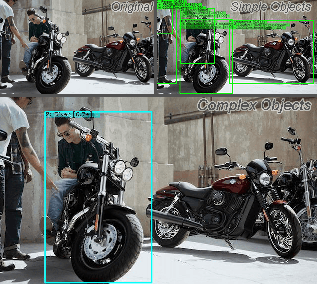
In addition to the <AttributeLib> and <SimpleObjectBase> tags shown in the previous example, <RelationLib> and <ComplexObjectBase> have been added, that store descriptions of relations and complex objects, respectively. This description is an example where parts of one complex object are recognized by different networks. The figure below shows the original image, separately recognized simple objects, and the result of the complex recognition.
Constructing complex objects from parts (source: pinterest)
As you can see in the figure, the system correctly identified the biker, although there are several people and motorcycles in the image.
Note: We will explain what the number 0.74 means for a given object in a bit. Before we do that, let’s look at a more complex example.
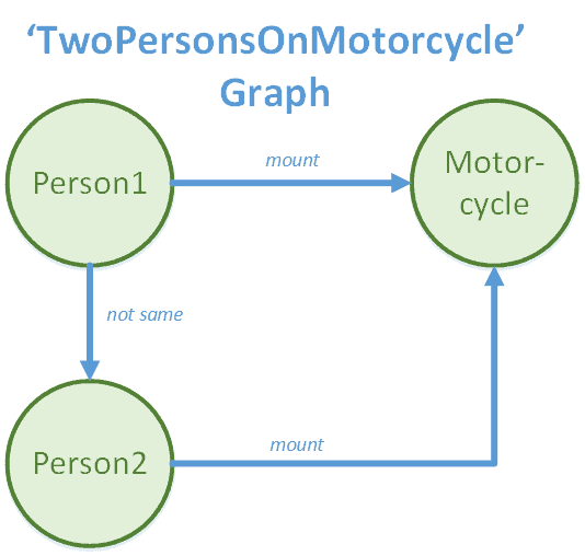
Example 3. The problem statement of the previous example is not particularly difficult. For example, self-driving car systems should be able to recognize motorcyclists as a separate class, and most developers in this area probably do this. Let’s now try to set the problem in such a way so as to recognize a situation when two people are riding a motorcycle at once. Another “person” object is added to the previous graph, linked by a “mount” relationship to the same “motorcycle”. However, in view of the specifics of the problem of finding an isomorphic subgraph, it is also necessary to indicate to the system that both people must be different.
Graph representation of a complex object when two people ride the same motorcycle
For the system, such a view will be described as follows:
<?xml version="1.0" ?>

<AttributeLib>
  ...
</AttributeLib>

<SimpleObjectBase>
  ...
</SimpleObjectBase>

<RelationLib>
   ...
   <RelationShip Type="SpaceLeft" Name="left"/>
   <RelationShip Type="SpaceRight" Name="right"/>

   <RelationShip Type="LogicOr" Name="not_same" A="left" B="right"/>

</RelationLib>

<ComplexObjectBase>

     <ComplexObject ID="3" Name="TwoPersonsOnMotorcycle">
        <SimpleObject Class="Person" InnerName="Person1"/>
        <SimpleObject Class="Person" InnerName="Person2"/>
        <SimpleObject Class="Motorcycle" InnerName="Motorcycle"/>

        <Relation Obj1="Person1" Obj2="Motorcycle" Relationship="mount"/>
        <Relation Obj1="Person2" Obj2="Motorcycle" Relationship="mount"/>

        <Relation Obj1="Person1" Obj2="Person2" Relationship="not_same"/>

        <Filter Type="NMS" threshold="0.5"/>
    </ComplexObject>

</ComplexObjectBase>
In the XML description above, I replaced with … the unchanged parts with the previous example to save space. The image below also shows the original picture, the result of recognizing simple objects and complex ones.
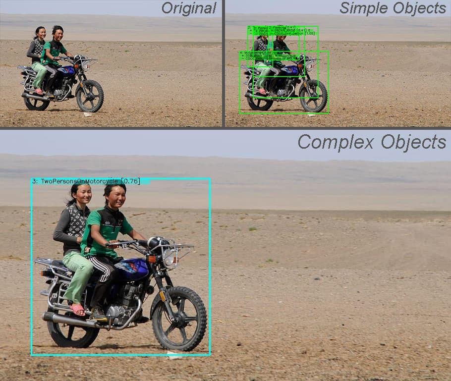
Constructing another complex object from the parts (source: pxfuel)
You may have noticed that both in this example and in the previous one in the description of a complex object there was a line:
<Filter Type="NMS" threshold="0.5"/>
It means that the Nonmax Suppression operation, which is widespread in computer vision, is applied to the recognition result, which allows filtering out all detections in one area except for the one with the highest score. Several detections with this approach occur for two reasons. The first one is multiple triggers of the detector of simple objects (for example, the detector recognized three people in the image above). The second is the duality of the description – in the example, there are objects “Person1” and “Person2”, and each of them can be the girl or boy in the image, so the system gives two results: one where “Person1” is the boy and “Person2” is the girl, and the other is vice versa.
Soft mode detection & tracking
The examples above illustrate the so-called “hard detection mode” that recognizes only objects that fully match the given description. However, it may be required to get a list of similar objects to the given one in some situations. For example, if we are looking for a red cup as in the first example, then just a cup or just a red spot, in a sense, is similar to the desired object. Perhaps, this is the required object; just one attribute detector worked incorrectly. I define the degree of similarity between simple objects as:
Where pi are the scores given by the attribute detectors, ki is the manually set significance coefficients. We normalize the degree of similarity to the interval [0, 1] (provided that pi also complies with this normalization). The score is 1 when the objects are the same and 0 when there are no common features. This value is shown in square brackets after a simple object’s name in all examples below. We can use this knowledge in different ways. For example, a robot looking for some object in a room can move closer to the object detected by a simpler attribute (color, shape) to “examine” it in more detail.
The most general formulation of such a question is the tracking procedure. It is required in video data recognition systems and is designed to match objects in frame t with objects in frame t+1. In our system, this is done similarly to the detecting simple objects procedure. However, soft recognition also makes it possible to “remember” that the object had a higher degree of similarity before the recognition accuracy deteriorates.
Example 4. Consider the example of recognizing a typical computer mouse, but in addition to the attribute of the concept identified by the neural network, we will also add a color attribute. In this case, it is a roughly tuned black color detector. Next, we will configure the system so that for the recognition, it is sufficient to have only a recognized concept, but at the same time, if only the color attribute is recognized in the area where the concept attribute was previously observed, then we continue to consider that object a mouse. In the video below, the camera is drifting away, and over time the neural network detector loses the object. Color filtering gives a fair amount of false positives, but the combination of these attributes through soft tracking allows tracking an object robustly.
We can also implement soft recognition for complex objects. For finding isomorphic subgraphs to work with uncertainties, I had to modify the input data by adding fake objects and connections to the observation graph.
In the picture below, the object from the example 3 is looked for in the picture from the example 2 in soft mode with zero threshold of degree of similarity.
Soft mode detection for the ‘two people on a motorcycle’ complex object.
As you can see, there are a lot of positives, including the ones with zero degrees of similarity, which is determined in the case of a complex object by the following formula:
where kr is the coefficient of significance of the relation, kr(o) is the coefficient of significance of the object connected by the relation r, Dc is the degree of confidence of simple objects (previous formula). So one motorcycle looks like two people on a motorcycle with the degree of 0, when one person on a motorcycle looks more like a given object. The degree of similarity for complex graphs is also calculated in the hard detection mode. All the examples above indicate it in square brackets after the complex object name.
At the moment, soft tracking for complex objects is under development. Localization of mobile robots is another practical application of this approach that we are currently developing. Semantic indoor mapping is an actively developing area within the Spatial AI direction. Maps, which consist of named objects, allow taking human-machine interaction to a new level, creating systems that allow you to give commands to robots in a natural language, for example, “sweep under the table in the kitchen” or “fetch a blue dress from the closet” etc.
Conclusion
In conclusion, I want to list the capabilities of the system I am creating, the scope, its advantages, and some of the challenges that face it.
The system allows:
- combining various attributes within one simple object, allowing you to precisely tune to a specific type;
- combining simple objects into complex ones, specifying the relationship between them;
- performing recognition in soft mode, in which the system can give information about similar objects (both simple and complex) to the desired one and specifying a degree of confidence;
- performing tracking for simple objects in a soft recognition mode, increasing the stability of recognition.
And:
- for simple objects, classic tracking approaches are available;
- it is possible to add various filters to system elements;
- it is possible to work with both RGB images and a depth map obtained, for example, from a stereo camera.
I developed this approach for ROS because robotics is my primary area of interest. The solution is publicly available on GitHub and has documentation in two languages. Also, the ROS version and the main unit dealing with recognition contain many utilities that allow you to configure the parameters of some detectors.
There is also a graphical QT application for debugging the main library, which is also publicly available on GitHub. The application has been tested only on Linux Ubuntu, but there are plans to adapt it for Windows shortly.
The solution’s core uses OpenCV 4.2.0 since this version comes with ROS Noetic – the latest version of the framework (besides ROS2).
The system has the following benefits:
- the possibility of rapid prototyping of the object recognition system, combining ready-made methods in different ways;
- the versatility of the architecture makes it easy to expand the system with new methods;
- object recognition with a degree of similarity.
On the other hand, there are several challenges:
- like most classical computer vision methods, this approach is highly sensitive to manually adjusted parameters;
- soft tracking algorithms work well only when moving objects smoothly;
- many parts of the source code still need optimization.
Links to different parts of the solution:
- common group on GitHub: https://github.com/Extended-Object-Detection-ROS
- solution core: https://github.com/Extended-Object-Detection-ROS/lib
- static examples from this post: https://github.com/Extended-Object-Detection-ROS/opencv_blog_olympics_examples (but slightly modified)
- English documentation: https://github.com/Extended-Object-Detection-ROS/wiki_english/wiki
- Simple console application: https://github.com/Extended-Object-Detection-ROS/dummy_console_app
- QT graphic user interface application: https://github.com/Extended-Object-Detection-ROS/qt_gui_eod
- ROS-interface package: https://github.com/Extended-Object-Detection-ROS/extended_object_detection
- YouTube channel with some examples: https://www.youtube.com/channel/UCrZtFXAhxJIyk-T3d9-GLhw
References
[1] A. Farhadi, I. Endres, D. Hoiem, and D. Forsyth, “Describing objects by their attributes,” in 2009 IEEE Conference on Computer Vision and Pattern Recognition, Jun. 2009, pp. 1778–1785, doi: 10.1109/CVPR.2009.5206772.
[2] O. Russakovsky and L. Fei-Fei, “Attribute Learning in Large-Scale Datasets,” in Trends and Topics in Computer Vision, 2012, pp. 1–14.
[3] Z. Zheng, A. Sadhu, and R. Nevatia, “Improving Object Detection and Attribute Recognition by Feature Entanglement Reduction,” Aug. 2021, [Online]. Available: http://arxiv.org/abs/2108.11501
[4] S. Banik, M. Lauri, and S. Frintrop, “Multi-label Object Attribute Classification using a Convolutional Neural Network,” Nov. 2018, [Online]. Available: http://arxiv.org/abs/1811.04309
[5] Z. Nan, Y. Liu, N. Zheng, and S.-C. Zhu, “Recognizing Unseen Attribute-Object Pair with Generative Model,” Proc. AAAI Conf. Artif. Intell., vol. 33, pp. 8811–8818, Jul. 2019, doi: 10.1609/aaai.v33i01.33018811.
[6] C. H. Lampert, H. Nickisch, and S. Harmeling, “Learning to detect unseen object classes by between-class attribute transfer,” in 2009 IEEE Conference on Computer Vision and Pattern Recognition, Jun. 2009, pp. 951–958, doi: 10.1109/CVPR.2009.5206594.
[7] Y. Sun, L. Bo, and D. Fox, “Attribute based object identification,” in 2013 IEEE International Conference on Robotics and Automation, 2013, pp. 2096–2103, doi: 10.1109/ICRA.2013.6630858
[8] C. Ye, Y. Yang, C. Fermuller, and Y. Aloimonos, “What Can I Do Around Here? Deep Functional Scene Understanding for Cognitive Robots,” Jan. 2016, [Online]. Available: http://arxiv.org/abs/1602.00032
[9] X. Chang, P. Ren, P. Xu, Z. Li, X. Chen, and A. Hauptmann, “Scene Graphs: A Survey of Generations and Applications,” Mar. 2021, [Online]. Available: http://arxiv.org/abs/2104.01111
[10] J. Johnson, A. Gupta, and L. Fei-Fei, “Image Generation from Scene Graphs,” Apr. 2018, [Online]. Available: http://arxiv.org/abs/1804.01622
[11] J. Zhou et al., “Graph Neural Networks: A Review of Methods and Applications,” Dec. 2018, [Online]. Available: http://arxiv.org/abs/1812.08434













100K+ Learners
Join Free OpenCV Bootcamp3 Hours of Learning