3D LiDAR Visualization using Open3D: A Case Study on 2D KITTI Depth Frames for Autonomous Driving

3D LiDAR sensor (or) 3-dimensional Light Detection and Ranging is an advanced light-emitting instrument that has the ability to perceive the real-world in a 3-dimensional space, just as we humans do. This technology has particularly revolutionized the fields of earth observation, environmental monitoring, reconnaissance, and now autonomous driving. Its ability to deliver accurate and detailed data has been instrumental in advancing our understanding and management of the environment and natural resources.

In this definitive research article, we will comprehensively focus on visualizing 3D LiDAR sensor data and try to gain an in-depth understanding of the 3D point cloud representation system for self-driving autonomy. Stay tuned for the zenith of this article – the experimental results showcasing 3D point-cloud visualization.

To see the results, you may SCROLL BELOW to the concluding part of the article or click here to see the visualization results.

Evolution and Impact of Laser Technology

In 1960, Theodore Maiman and his team at Hughes Research Laboratory made a groundbreaking discovery by illuminating a ruby rod with a high-power flash lamp, thereby generating the first laser beam (Xin Wang et al. [1]). This beam of coherent light marked a significant advancement in technology due to its exceptional brightness, precision, and resistance to interference. Laser technology, with its inherent attributes of superior brightness, directivity, and anti-jamming capabilities, has since become indispensable in the field of range measurement. Compared to traditional measurement methods, laser-based techniques offer heightened precision and resolution. They are also characterized by their compact size, ease of use, and ability to operate under various conditions, making them invaluable in a wide range of applications.

At first, laser ranging was predominantly used in military and scientific research instruments, with its application to industrial instruments being relatively rare. This limited usage was primarily due to the high cost of laser ranging sensors, which were typically priced in the thousands of dollars. This prohibitive cost was a significant barrier to a broader adoption. However, with substantial advancements in technology, the scenario has changed dramatically. The cost of these sensors has decreased significantly, now amounting to only a few hundred dollars. This price reduction has positioned laser ranging as a viable and cost-effective solution for various long-range inspection applications in the future.

Diverse types of laser ranging systems have been developed, including single-beam, two-dimensional, and three-dimensional systems. The single-beam system is designed for distance measurement, the two-dimensional system for scanning planes, and the three-dimensional system for determining coordinates and profiling.

The high precision, rapid speed, and strong anti-interference capabilities of these advanced laser ranging systems have attracted considerable attention in the research and application spheres. As a result, many researchers from universities and institutes world-wide are actively engaged in exploring and enhancing this technology.

Crucial Role of 3D LiDAR in Autonomous Driving

LiDAR sensors play a critical role in increasing the significance of the autonomy component in advanced driver assistance systems due to their ability to create accurate, real-time 3D maps of the vehicle’s surroundings. Here are a few specific reasons that prove its significance:

• High-Resolution Spatial Mapping: 3D LiDAR sensors emit laser beams to measure distances and then use the reflected light to create detailed three-dimensional maps of the environment. This high-resolution spatial mapping is essential for autonomous vehicles to navigate complex environments safely.
• Range and Precision: These systems are highly accurate and capable of precisely detecting objects and their dimensions. They are effective over a range of distances, allowing autonomous vehicles to detect objects near and far, which is crucial for path planning and obstacle avoidance.
• All-Weather Performance: Like any other sensor 3D LiDAR can be affected by extreme weather conditions. However, it performs reliably in various environments and weather conditions, including low-light scenarios where cameras might struggle.
• Object Detection and Classification: It is not just about detecting objects; it also helps classify them based on size, shape, and behavior. This is crucial for autonomous vehicles to differentiate between various elements like pedestrians, other vehicles and static obstacles. 
• Real-Time Processing and Computation: These sensors can process data in real-time, providing immediate feedback to the autonomous vehicle’s system. This is vital for making quick decisions in dynamic driving scenarios.

Key Role of 3D Visualization in Analyzing 3D LiDAR Data

Analyzing LiDAR data is immensely significant, fundamentally transforming how we interpret and comprehend intricate spatial environments. This is crucial for the following  reasons:

• Detailed Environmental Representation: 3D visualization allows for the comprehensive representation of environments captured by LiDAR. It transforms raw data points into a visually coherent and interpretable three-dimensional model, offering a clear and detailed view of physical spaces.
• Enhanced Data Interpretation: Traditional 2D representations can obscure or flatten critical details about terrain and structures. 3D visualization, on the other hand, provides depth perception and spatial awareness, which are essential for accurately interpreting 3D LiDAR sensor data.
• Interactive Analysis: 3D visualization tools often allow users to interact with the data, such as zooming, panning, and rotating the view. This interactivity enhances the analysis by allowing users to explore the data from different angles and perspectives.

Cutting-Edge Research: Papers on 3D LiDAR Visualization Techniques

In this section, we will explore different implementations and use-cases where 3D visualization has helped to understand complex data and solve novel problems.

Xiohan Tu et al., [2] developed RobotNet, a lightweight deep learning model enhanced with depthwise and pointwise convolutions and an attention module, specifically designed for efficient and accurate recognition of overhead contact (OC) components in 3D LiDAR sensor data, targeting high-speed railway inspections. To augment its speed on embedded devices, RobotNet was further optimized by utilizing a compilation tool.

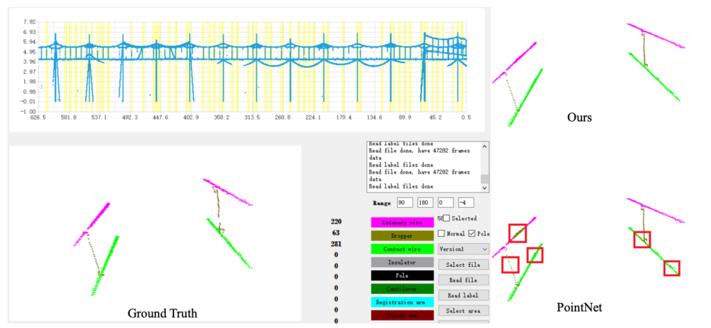
Complementing this, the team also engineered software capable of visualizing extensive point cloud data, including intricate details of OC components. Their extensive experiments demonstrated RobotNet’s superior performance in terms of accuracy and efficiency over other methods, marked by a significant increase in inference speed and reduced computational complexity.

The paper by Nicholas Crabb et al., [3] explores the use of LiDAR in mapping and interpreting natural and archaeological features, particularly focusing on its integration in geoarchaeological deposit models. The authors conduct a comprehensive review and quantitative evaluation of various visualization methods for LiDAR elevation models, specifically in archaeologically rich alluvial environments.

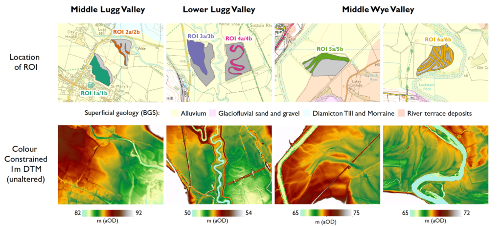
They found that due to the low-relief nature of temperate lowland floodplains, only a few visualization methods significantly enhance the detection of geomorphological landforms linked to the distribution of archaeological resources. The study concludes that a combination of Relative Elevation Models and Simple Local Relief Models is most effective, offering optimal integration with deposit models. While the research is centered on floodplain environments, the methodology and findings have broader applicability across various landscape contexts.

Jyoti Madake et al., [4] address the obstacle detection problem in computer vision, focusing on object detection using multiple modalities, specifically combining camera and LiDAR data, primarily utilized in robotics and automation. It highlights LiDAR’s effectiveness in creating point clouds essential for object detection and employs various deep learning models for this purpose.

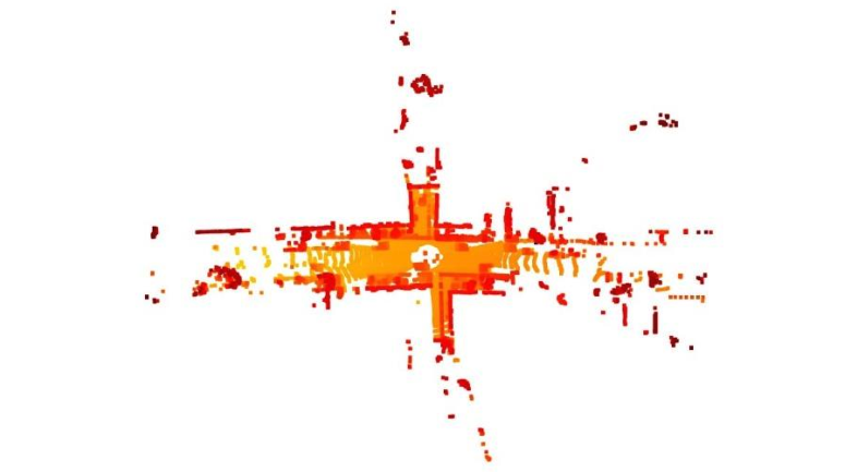
The authors proposed a vehicle detection system using camera and LiDAR data, processed with the Open3D library. Techniques like Random Sample Consensus (RANSAC) and Density-Based Spatial Clustering of Applications with Noise (DBSCAN) are applied for visualization and clustering in LiDAR point clouds. This study aims to detect vehicles as clusters, utilizing major datasets such as KITTI, Waymo Open Dataset, and the Lyft Level 5 AV Dataset.

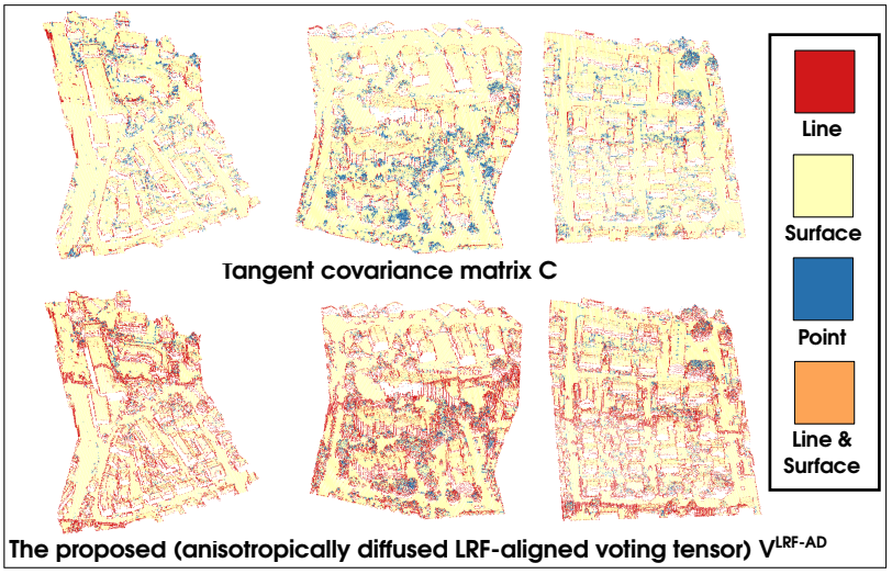
Jaya Sreevalsan’s [5] research focuses on 3D analysis of airborne LiDAR datasets, specifically exploring the role of visual analytics in point cloud processing. They delve into two main application scenarios: unsupervised classification of point clouds and local geometry analysis. The study discusses structural (points, lines, surfaces) and semantic (buildings, ground, vegetation) classification of point clouds. Emphasizing urban regions, the research utilizes datasets where these object classes are prevalent. The team develops a local geometric descriptor using tensor voting and gradient energy tensor, offering an alternative to the conventional covariance matrix approach. Her work demonstrates the benefits of incorporating user interactivity and visualizations into data science workflows, enabling effective exploration of large-scale airborne LiDAR point clouds.

Methodology

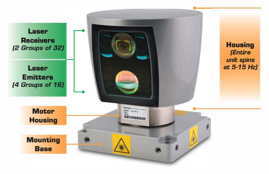
Velodyne HDL-64E S2 3D LiDAR Sensor

The latest S2 version of the HDL-64E boasts improved accuracy and a higher data rate compared to its predecessor, marking a notable evolution in the product line.

Highlights

• The Velodyne HDL-64E S2 features a comprehensive 360-degree horizontal and 26.8-degree vertical Field of View, providing extensive environmental data capture with over 1.3 million points per second. 
• Its innovative design includes 64 fixed-mounted lasers in a single rotating unit, enhancing reliability and point cloud density compared to traditional LiDAR systems.
• Equipped with high-performance specifications, the HDL-64E S2 offers superior distance accuracy and effective detection range, ideal for diverse environmental conditions.
• The sensor’s proven track record in prestigious events like the DARPA Grand and Urban Challenges underscores its effectiveness and reliability in real-world autonomous vehicle applications.

The HDL-64E S2 has 64 lasers/detectors, providing a 360-degree azimuth field of view and a 0.08-degree angular resolution. Its vertical field of view spans 26.8 degrees, with 64 equally spaced angular subdivisions. The sensor boasts less than 2 cm distance accuracy and a range of up to 120 meters for detecting cars and foliage, making it highly effective in diverse environments. The sensor operates efficiently within a temperature range of -10° to 50° C and has a storage temperature range of -10° to 80° C.

Designed with user convenience in mind, the HDL-64E S2 utilizes a Class 1 eye-safe laser with a 905 nm wavelength. It features dynamic laser power selection for an expanded dynamic range and delivers its output via 100 MBPS UDP Ethernet packets. The sensor’s mechanical aspects include a power requirement of 15V ± 1.5V at 4 amps, a weight of less than 29 lbs, and environmental protection rated at IP67.

Description of the 2D KITTI Depth Frames Dataset

The KITTI dataset stands out as a pivotal resource in the domain of self-driving car research. It encompasses a comprehensive collection of data gathered from cameras, LiDAR, and other sensors mounted on a vehicle traversing through diverse street environments and scenarios. This rich compilation provides an extensive range of real-world contexts, crucial for developing and testing autonomous driving technologies. The Velodyne LiDAR sensor shown in the previous section was used to capture data for this specific dataset.

Highlights

• Transformation of Complex LiDAR Data:  The KITTI LiDAR-Based 2D Depth Images dataset features a unique transformation of 360-degree LiDAR frames into a 2D format. This process involves ‘unwrapping’ the cylindrical LiDAR frames, making the complex three-dimensional data more accessible and simpler to process in two dimensions.
• Depth Information in Pixels: In this dataset, each pixel of the 2D depth images represents the distance from the 3D LiDAR sensor to objects in the environment. This approach maintains the integrity of the original LiDAR data, effectively capturing the same scenes but in a more processable format.
• High Vertical Resolution for Detailed Scanning: The dataset sets a high vertical resolution of 64, reflecting the number of laser beams utilized by the 3D LiDAR sensor. This high resolution ensures detailed scanning and mapping of the surroundings, crucial for precise environmental modeling.

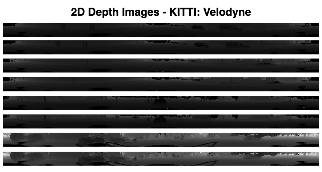
In this specific subset, the focus is on 2D depth images derived from the LiDAR frames of the KITTI dataset. These images represent a transformation of the original 360-degree LiDAR frames, which are typically presented in a cylindrical format around the sensor. The conversion process essentially involves ‘unwrapping’ the cylindrical LiDAR frames into a 2D plane, thereby translating the complex three-dimensional data into a more accessible two-dimensional format.

Each pixel in these 2D depth images corresponds to the distance between the LiDAR sensor and the objects reflected in the laser beams, effectively capturing the same scenes as the original LiDAR frames but in a format that is simpler to process. The vertical resolution of these images, set at 64 in this dataset, indicates the number of laser beams used by the LiDAR sensor for scanning the surroundings.

The utility of these 2D depth images extends across various applications, including segmentation, detection, and recognition tasks. They provide a bridge between the advanced capabilities of LiDAR technology and the extensive body of existing computer vision literature focused on 2D image analysis. This makes the KITTI LiDAR-Based 2D Depth Images dataset not only a valuable asset for autonomous vehicle research but also a versatile tool for exploring a wide array of computer vision challenges and opportunities.

The Open3D Visualization Tool

Highlights

• Versatile and Efficient 3D Data Processing: Open3D is a comprehensive open-source library that provides robust solutions for 3D data processing. It features optimized back-end architecture for efficient parallelization, making it ideal for handling complex 3D geometries and algorithms. 
• Realistic 3D Scene Modeling and Analysis: The library offers specialized tools for scene reconstruction and surface alignment, which are fundamental in creating accurate 3D models. Its implementation of Physically Based Rendering (PBR) ensures that visualizations of these 3D scenes are not only precise but also strikingly realistic, greatly enhancing the user’s experience and the applicability of the tool in various professional scenarios.
• Cross-Platform Compatibility: It supports various compilers like GCC 5.X, XCode 10+, and Visual Studio 2019, ensuring seamless operation across Linux, OS X, and Windows. It offers simple installation processes through conda and pip, facilitating quick and hassle-free setup for users.

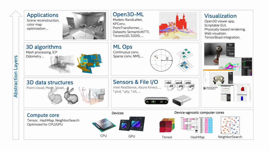
Developed from the ground up, Open3D focuses on a lean and purposeful selection of dependencies, making it a lightweight yet powerful tool in 3D data processing. Its cross-platform compatibility is a key feature, allowing for straightforward setup and compilation on various operating systems with minimal effort. Its codebase is characterized by its cleanliness, consistent styling, and transparent code review process, reflecting its commitment to high-quality software engineering practices.

Adding to its realism in visualization, Open3D incorporates Physically Based Rendering (PBR), which brings a new level of realism to 3D scene visualization. Its comprehensive 3D visualization capabilities allow for an interactive exploration of 3D data, enhancing user engagement and understanding. Additionally, it includes Python bindings, providing a user-friendly and powerful interface for scripting and rapid prototyping, making it an ideal choice for both novice and experienced practitioners in the field.

The library’s utility and effectiveness are evidenced by its use in numerous published research projects and active deployment in cloud-based applications. Open3D encourages and welcomes contributions from the global open-source community, fostering a collaborative and innovative development environment. This makes Open3D not just a tool for 3D data processing but also a platform for collaborative innovation in the field of 3D data analysis and visualization.

3D Point-Cloud Visualization – Code Walkthrough

In this section, we will explore the various processes involved in visualizing the KITTI 3D LiDAR sensor scans dataset, and also generate a 3D point cloud representation of the same. You can download the code in this article by clicking on the Download Code button.

Click here to download the source code to this post

Load and Read 2D Depth Image

This code snippet defines a function `load_depth_image`, which is written to read and process 2D depth images.

# Read the 2D Depth Image
def load_depth_image(file_path):
    # Load the depth image
    depth_image = plt.imread(file_path)
    depth_image_scaling_factor = 250.0
    # Assuming the depth image is normalized, we may need to scale it to the actual distance values
    # This scaling factor is dataset-specific; you'll need to adjust it based on the KITTI dataset documentation
    depth_image *= depth_image_scaling_factor
    
    return depth_image

Upon execution, the function performs the following operations:

• Image Loading: Utilizes `plt.imread`, a function from the `matplotlib` library, to load the image located at the specified `file_path`. This step reads the image data and stores it in the variable `depth_image`.
• Depth Image Scaling: The code sets a `depth_image_scaling_factor’. This scaling factor is crucial for converting the normalized depth values in the image to actual distance measurements, which represent the real-world distance from the 3D LiDAR sensor to the objects in the scene. The scaling factor’s value is dataset-specific and, in this case, is presumably tailored to suit the characteristics of the KITTI dataset.
• Normalization Adjustment: This adjustment transforms the normalized values into a more meaningful representation of actual distances, enhancing the utility of the depth data for further processing and analysis.

Process Multiple Frames of 2D Depth Frames

This code snippet defines a function `load_and_process_frames`, which is designed to process a series of 2D depth image files from a specified directory, converting them into point cloud data.

def load_and_process_frames(directory):
    point_clouds = []
    for filename in sorted(os.listdir(directory)):
        if filename.endswith('.png'):  # Check for PNG images
            file_path = os.path.join(directory, filename)
            depth_image = load_depth_image(file_path)
            point_cloud = depth_image_to_point_cloud(depth_image)
            point_clouds.append(point_cloud)
    return point_clouds

The function is particularly useful in contexts where multiple depth images need to be processed and analyzed collectively. Here’s a breakdown of its functionality:

• Point Cloud List Initialization: This function takes one argument, `directory`, which specifies the path to the folder containing the depth image files. A list named `point_clouds` is initialized to store the point cloud data converted from each depth image. 
• Directory File Iteration: The `sorted(os.listdir(directory))` ensures that the files are processed in alphabetical (or numerical) order, which is particularly important for sequential data like frames in a video or 3D LiDAR scan.
• File Type Check: Within the loop, the function checks if the current file is a PNG image (`filename.endswith(‘.png’)`). This is crucial to ensure that only depth image files are processed.
• Depth Image Processing: For each PNG image file, the function constructs its full path (`file_path`) and then loads the depth image using a previously defined function `load_depth_image`. This function is expected to read the depth image and possibly perform some initial processing.
• Point Cloud Conversion: The loaded depth image is then converted into a point cloud using another function, named `depth_image_to_point_cloud`. This function is expected to take the depth information from the 2D image and transform it into a 3D point cloud representation, and the resulting point cloud from each image is appended to the `point_clouds` list. After all PNG images in the directory have been processed, the function returns the list of point clouds.

Converting 2D Depth Frames to 3D LiDAR Point Cloud

The function `depth_image_to_point_cloud` is designed to convert a 2D depth image into a 3D point cloud.

def depth_image_to_point_cloud(depth_image, h_fov=(-90, 90), v_fov=(-24.9, 2.0), d_range=(0,100)):
    # Adjusting angles for broadcasting
    h_angles = np.deg2rad(np.linspace(h_fov[0], h_fov[1], depth_image.shape[1]))
    v_angles = np.deg2rad(np.linspace(v_fov[0], v_fov[1], depth_image.shape[0]))
    # Reshaping angles for broadcasting
    h_angles = h_angles[np.newaxis, :]  # Shape becomes (1, 1440)
    v_angles = v_angles[:, np.newaxis]  # Shape becomes (64, 1)
    # Calculate x, y, and z
    x = depth_image * np.sin(h_angles) * np.cos(v_angles)
    y = depth_image * np.cos(h_angles) * np.cos(v_angles)
    z = depth_image * np.sin(v_angles)
    # Filter out points beyond the distance range
    valid_indices = (depth_image >= d_range[0]) & (depth_image <= d_range[1])
    
    # Apply the mask to each coordinate array
    x = x[valid_indices]
    y = y[valid_indices]
    z = z[valid_indices]
    # Stack to get the point cloud
    point_cloud = np.stack((x, y, z), axis=-1)
    return point_cloud

This conversion is particularly useful in the context of LiDAR data processing, where depth information from a 2D image is transformed into a spatially informative 3D format. The function’s operations are as follows:

• Angle Adjustment for Broadcasting: This function accepts four parameters: `depth_image`, which is the input 2D depth image, `h_fov` and `v_fov` representing the horizontal and vertical fields of view (FoV) respectively, and `d_range` specifying the distance range for filtering the depth data. The horizontal (`h_angles`) and vertical (`v_angles`) angles based on the provided fields of view. It uses `np.linspace` to create evenly spaced angles within the specified FoV ranges and then converts these angles from degrees to radians using `np.deg2rad`.
• Reshaping Angles: The horizontal angles are reshaped to have a shape of (1, number of columns in depth image) and the vertical angles to (number of rows in depth image, 1). This reshaping facilitates broadcasting when performing element-wise operations with the depth image.
• 3D Coordinate Computation: x, y, and z coordinates of each point in the point cloud are computed using trigonometric operations. The depth values from the depth image are used along with the sine and cosine of the calculated angles to determine the position of each point in 3D space.
• Distance Range Filtering: The points that do not fall within the specified distance range (`d_range`) are filtered out. This is achieved by creating a mask based on the depth values and applying it to each coordinate array (x, y, z).
• 3D Point Cloud Construction: Valid x, y, and z coordinates are stacked along a new axis to form the final 3D point cloud. This results in an array where each element represents a point in 3D space. Finally, the computed point cloud is now in a format suitable for 3-dimensional visualization and analysis.

Simulate Point Cloud Representation

The `animate_point_clouds` function is a Python routine designed to animate a sequence of 3D point clouds using the Open3D library.

def animate_point_clouds(point_clouds):
    vis = o3d.visualization.Visualizer()
    vis.create_window()
    # Set background color to black
    vis.get_render_option().background_color = np.array([0, 0, 0])
    # Initialize point cloud geometry
    point_cloud = o3d.geometry.PointCloud()
    point_cloud.points = o3d.utility.Vector3dVector(point_clouds[0])
    vis.add_geometry(point_cloud)
    frame_index = 0
    last_update_time = time.time()
    update_interval = 0.25  # Time in seconds between frame updates
    while True:
        current_time = time.time()
        if current_time - last_update_time > update_interval:
            # Update point cloud with new data
            point_cloud.points = o3d.utility.Vector3dVector(point_clouds[frame_index])
            vis.update_geometry(point_cloud)
            # Move to the next frame
            frame_index = (frame_index + 1) % len(point_clouds)
            last_update_time = current_time
        vis.poll_events()
        vis.update_renderer()
        if not vis.poll_events():
            break
    vis.destroy_window()

This function is particularly useful for visualizing dynamic 3D data, such as LiDAR scans or time-varying 3D simulations. Here is a detailed breakdown of its functionality:

• Visualization Setup: The function `animate_point_clouds` takes a single argument, `point_clouds`, which is expected to be a list of point cloud data. Each element in this list represents a distinct frame of the point cloud animation. It then initializes an Open3D Visualizer object (`vis`) and creates a new window for rendering the point cloud animation. The background color of the visualizer is set to black (`np.array([0, 0, 0])`), enhancing the visibility of the point cloud frames.
• 3D Point Cloud Initialization: A new Open3D PointCloud object (`point_cloud`) is created. The points for this point cloud are set to the first frame in the `point_clouds` list, preparing it for the initial display. The initialized point cloud is added to the visualizer. 
• Simulation Loop: `frame_index` tracks the current frame being displayed, `last_update_time` records the last time the frame was updated, `update_interval` sets the duration (in seconds) between frame updates, and the `while True` loop continuously updates the point cloud being displayed, cycling through the frames in the `point_clouds` list. The update occurs only if the elapsed time since the last update exceeds `update_interval`.
• 3D Point Cloud Updation: Within the loop, the point cloud’s points are updated to the current frame’s data, and the geometry is updated in the visualizer.
• Event Handling and Rendering: The `vis.poll_events()` and `vis.update_renderer()` calls handle user interactions and update the visualizer’s rendering, respectively.
• Simulation Termination: The loop breaks and exits if `vis.poll_events()` returns False, indicating that the visualizer window has been closed. Finally, the visualizer window is closed with `vis.destroy_window()`.

Run Visualization

This final code snippet provides a workflow for loading, processing, and simulating a series of 2D depth images into 3D point clouds using functions defined earlier in the script.

# Directory containing the depth image files
directory = 'archive/2011_09_30_drive_0028_sync/2011_09_30_drive_0028_sync/2011_09_30/2011_09_30_drive_0028_sync/velodyne_points/depth_images'
# Load and process the frames
point_clouds = load_and_process_frames(directory)
# Simulate the point clouds
animate_point_clouds(point_clouds)

Here’s a detailed description of each step:

• Directory Path Definition: The variable `directory` is assigned a string that specifies the path to a folder containing depth image files. In this case, the path points to a nested directory structure typical of the KITTI dataset, specifically targeting the depth images from the Velodyne LiDAR sensor.
• Loading and Processing Frames: The function `load_and_process_frames` is called with the `directory` variable as its argument. The function then iterates through the depth image files in the given directory, loading each image and converting it into a point cloud representation, and the resulting point clouds for each frame are aggregated into a list, `point_clouds`.
• Point Cloud Simulation: The function `animate_point_clouds` is then called with the `point_clouds` list. This is designed to simulate the sequence of point clouds, creating a visualization that represents the dynamic nature of the captured data. The simulation will be rendered in a window created by Open3D’s visualization tools, allowing for interactive exploration of the point cloud sequence.

Experimental Results and Discussion

In this section of the research article, we will explore the visualization results from this experiment. 

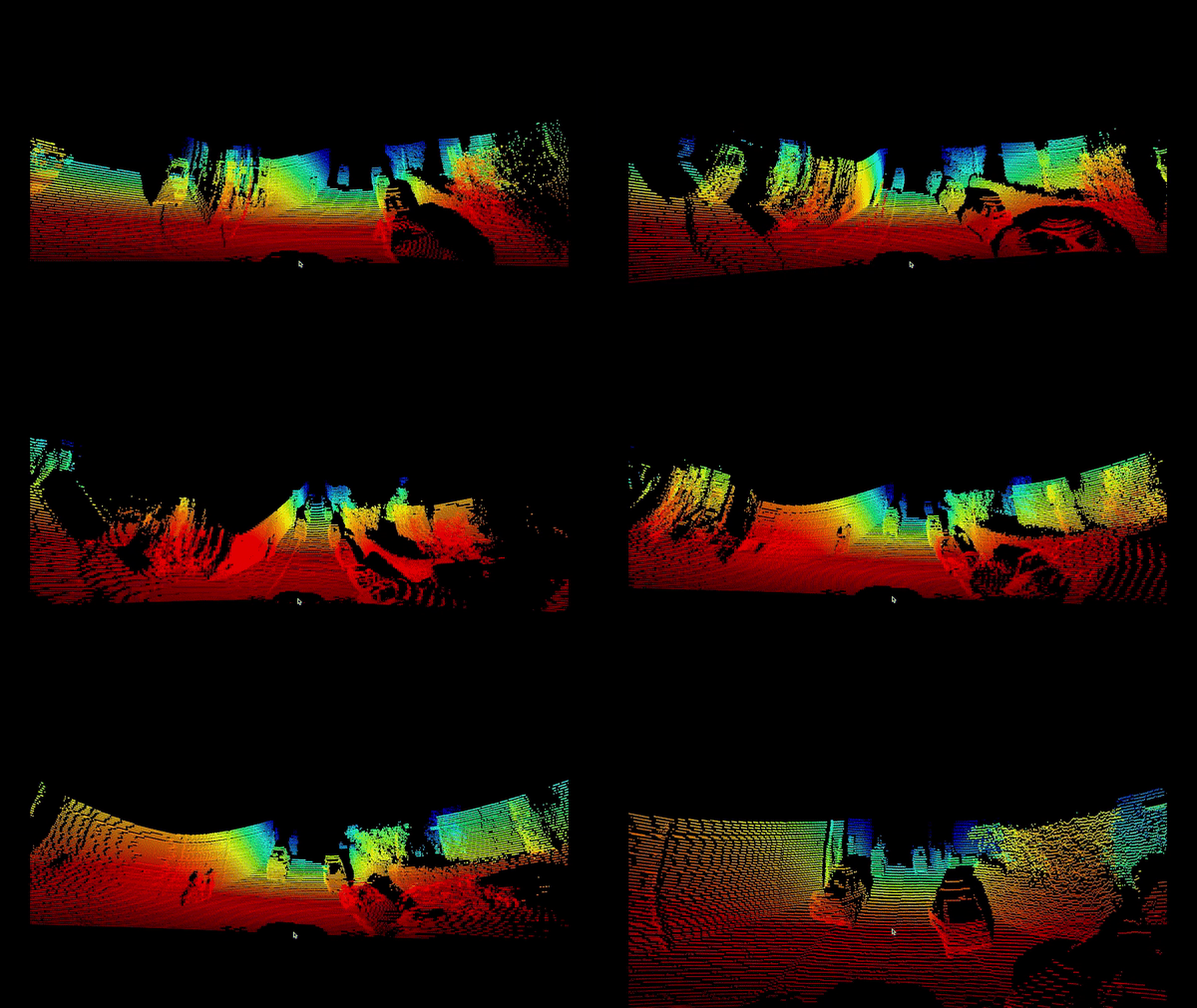
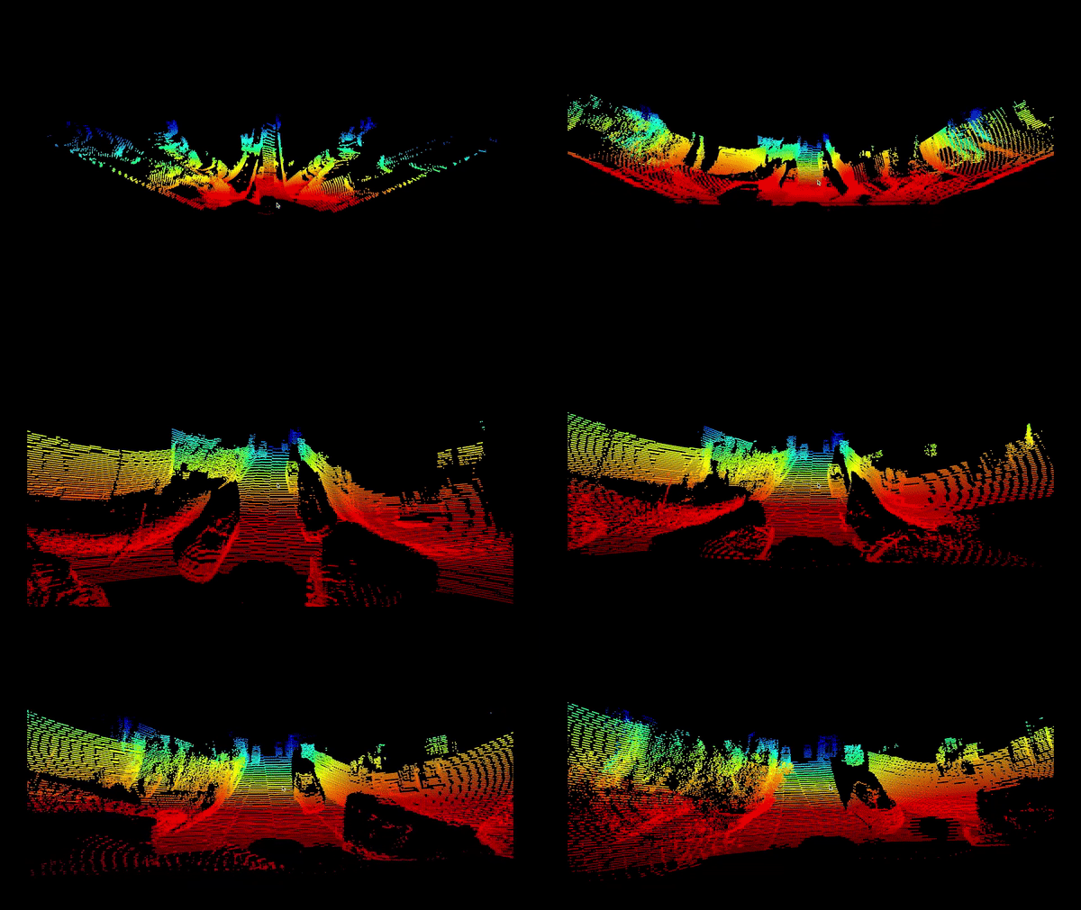
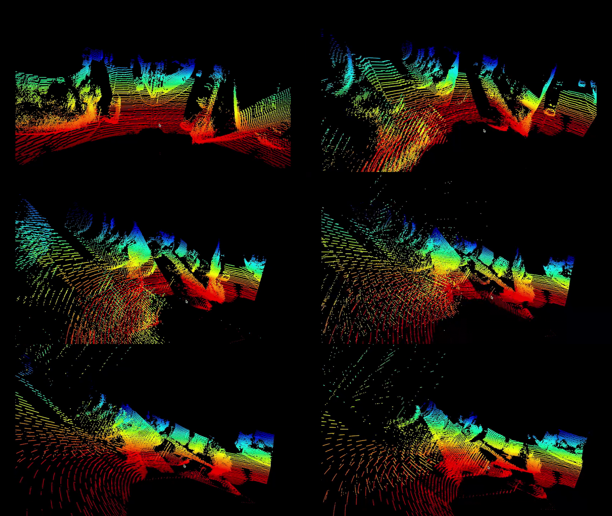
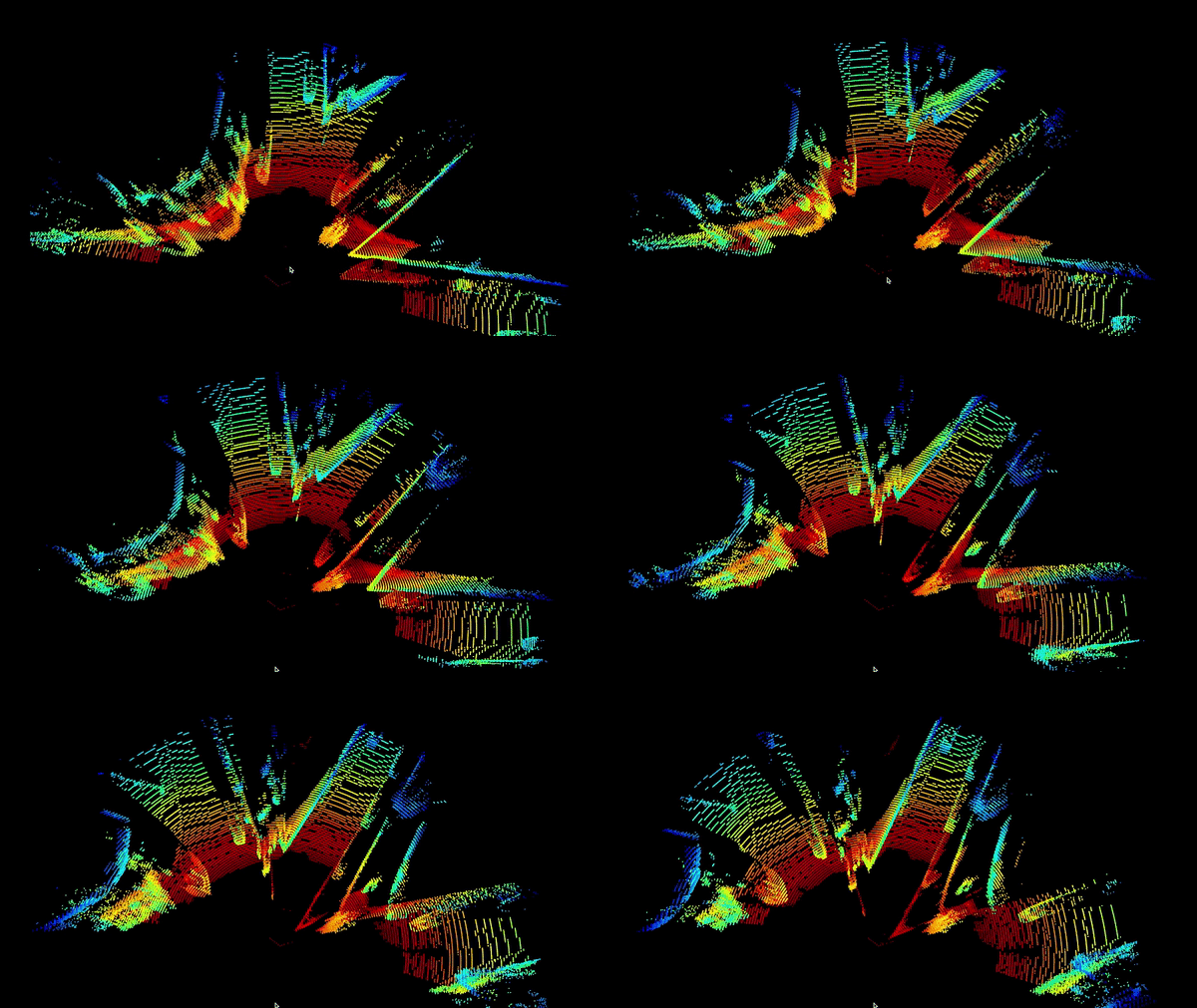
To enhance your understanding and engage hands-on with the code, take a walk through the code here.

The next step after 3D LiDAR visualization is to explore techniques to perform 3D LiDAR object detection. But if you’d further like to analyse the experimental results from this article, continue reading.

Analysis of 3D Point Cloud Representations

Based on the output 3D point cloud simulation, it is a colorized point cloud, a common method for visualizing three-dimensional LiDAR data. From the simulations shown above, several inferences can be made:

• Color Gradient: It usually corresponds to intensity or height, and shows variation across the point cloud. Warmer colors (reds and yellows) represent higher points or surfaces perpendicular to the sensor’s line of sight, whereas cooler colors (blues and greens) indicate lower areas or surfaces at an angle to the sensor.
• Data Density:  The density of the points is relatively high, indicating that the 3D LiDAR sensor used to capture this data has a high resolution, which is essential for detailed analysis.
• Sensor Position: In this simulation, the perspective of the point cloud suggests that the LiDAR sensor was positioned at ground level or on a vehicle, facing forward into the scene. But in this case, the sensor was placed on top of the car.  
• Dynamic Range: The broad range of colors also implies a significant dynamic range in the captured data, which can be helpful for distinguishing between different types of surfaces and objects.

3D LiDAR Comparison with 2D Depth Frames

Let’s now compare 2D depth maps and 3D point cloud simulations which involves understanding the fundamental differences in how they represent spatial data.

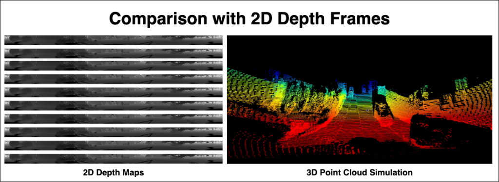
2D depth maps are essentially two-dimensional images where each pixel’s value represents the distance from the sensor to the nearest surface point along a direct line of sight. Depth maps are akin to grayscale images, where different shades correspond to varying distances. Generally require less computational power to process compared to 3D point clouds. They are more compatible with standard image processing techniques and algorithms. While they provide valuable distance information, they can lose context regarding the spatial arrangement and relation of objects in a scene.

3D point clouds are, in contrast, a point cloud, a collection of points in a three-dimensional coordinate system. Each point in a point cloud represents a tiny part of the surface of an object, providing a more holistic and spatially accurate representation of the scene. Processing point clouds often demands more computational resources. They require specialized algorithms for tasks like segmentation, object recognition, and 3D reconstruction. They also offer a more detailed and accurate representation of space and object geometry, and are better suited for tasks that require high fidelity spatial data.

Insights gained from 3D LiDAR for Autonomous Driving

In this subsection, let’s explore the insights gained from analyzing 3D point clouds and comparing them with 2D depth frames have significant implications for autonomous driving applications:

• Enhanced Environmental Perception: The color gradients and high data density in 3D point clouds provide a detailed and nuanced perception of the environment. In autonomous driving, this level of detail is crucial for accurately identifying and navigating complex urban landscapes, road conditions, and potential obstacles.
• Improved Obstacle Detection and Classification: The ability of 3D point clouds to depict the geometry and surface characteristics of objects allows for more effective obstacle detection and classification. This is vital for an autonomous vehicle’s decision-making process, particularly in differentiating between static objects (like lamp posts) and dynamic objects (like pedestrians).
• Depth Perception and Spatial Awareness: Unlike 2D depth maps, 3D point clouds offer superior depth perception and spatial awareness. This is critical for autonomous vehicles to understand their surroundings in three dimensions, which is essential for safe navigation and maneuvering.
• Sensor Fusion and Data Integration: This comparison also highlights the importance of integrating multiple sensor modalities. Combining the high-resolution spatial data from the 3D LiDAR sensor with the color and texture information from cameras can lead to a more comprehensive understanding of the vehicle’s surroundings.
• Path Planning and Navigation: The detailed information from 3D point clouds aids in more accurate path planning and navigation. Understanding the topography and layout of the environment ensures more efficient and safer route planning.

Future Work and Enhancements

Potential improvements in visualization techniques, particularly in the context of 3D point cloud data for autonomous driving applications, encompass a wide array of advancements aimed at enhancing clarity, accuracy, and user interaction. Key among these is the enhancement of real-time processing capabilities, enabling faster and more efficient interpretation of data crucial for immediate decision-making in autonomous vehicles. Integrating artificial intelligence and machine learning algorithms can lead to smarter visualization, facilitating automatic feature detection, anomaly identification, and predictive analysis. Increasing the resolution of point clouds can capture finer environmental details, crucial for precise object detection and scene interpretation. 

Advancements in color mapping and texturing techniques could provide more realistic and informative visualizations, especially when integrating LiDAR data with camera imagery to create richly textured 3D models. Developing interactive visualization tools will allow users to explore and analyze 3D point cloud data more intuitively, enhancing usability for those without specialized expertise. The incorporation of augmented and virtual reality technologies could offer immersive 3D environments, providing a more intuitive understanding of complex data sets. 

Apart from this, implementing advanced noise reduction and data filtering techniques is vital for enhancing the clarity of visualizations, aiding in the accurate interpretation of complex scenes. Addressing scalability and large data management will enable the handling of extensive datasets without performance compromise, crucial for analyzing vast areas or extended timeframes. Customizable visualization options, catering to various user needs and preferences, including adjustable viewpoints and rendering styles, would enhance the utility and accessibility of these tools. Lastly, ensuring that these visualization tools are accessible across different platforms, including mobile devices, and user-friendly to a broad user base, will significantly broaden their applicability and impact.

Conclusions

This research article has meticulously explored the visualization of 3D point cloud data and its comparison with 2D depth frames in the context of autonomous driving. Key findings from this study underscore the profound capabilities of 3D LiDAR sensor in providing detailed, high-resolution spatial data, which is paramount in the accurate mapping and interpretation of the environment for autonomous vehicles. The 2D depth images, while being less computationally intensive, sometimes fall short in capturing the complete spatial context that 3D point clouds offer, especially in complex urban landscapes. The impact of these findings on the field of autonomous driving is substantial. The enhanced perception and improved obstacle detection and classification capabilities provided by 3D point clouds are invaluable in advancing the safety, reliability, and efficiency of autonomous vehicles. 

References

[1] Xin Wang et al 2020 IOP Conf. Ser.: Earth Environ. Sci. 502 012008. https://iopscience.iop.org/article/10.1088/1755-1315/502/1/012008/pdf

[2] Tu, X.; Xu, C.; Liu, S.; Lin, S.; Chen, L.; Xie, G.; Li, R. LiDAR Point Cloud Recognition and Visualization with Deep Learning for Overhead Contact Inspection. Sensors 2020, 20, 6387. https://doi.org/10.3390/s20216387

[3] Crabb, N., Carey, C., Howard, A. J., & Brolly, M. (2023). Lidar visualization techniques for the construction of geoarchaeological deposit models: An overview and evaluation in alluvial environments. Geoarchaeology, 38, 420–444. https://doi.org/10.1002/gea.21959

[4] J. Madake, R. Rane, R. Rathod, A. Sayyed, S. Bhatlawande and S. Shilaskar, “Visualization of 3D Point Clouds for Vehicle Detection Based on LiDAR and Camera Fusion,” 2022 OITS International Conference on Information Technology (OCIT), Bhubaneswar, India, 2022, pp. 594-598, doi: 10.1109/OCIT56763.2022.00115.

[5]  Sreevalsan-Nair, J. (2018). Visual Analytics of Three-Dimensional Airborne LiDAR Point Clouds in Urban Regions. In: Sarda, N., Acharya, P., Sen, S. (eds) Geospatial Infrastructure, Applications and Technologies: India Case Studies. Springer, Singapore. https://doi.org/10.1007/978-981-13-2330-0_23