Comparing KerasCV YOLOv8 Models on the Global Wheat Data 2020

This article is a continuation of our series of articles on KerasCV. The previous article discussed fine-tuning the popular DeeplabV3+ model for semantic segmentation. In this article, we will shift our focus back to object detection. We will primarily use the popular Global Wheat Challenge released in 2020 on Kaggle by comparing KerasCV YOLOv8 models. 

Specifically, in this post, we will compare three detection models, namely:

• YOLOv8 small
• YOLOv8 medium
• YOLOv8 large

Finally, we will ensemble the predictions across these models to produce more efficient unified predictions using a popular technique called Weighted Boxes Fusion (WBF).

1. The Global Wheat Detection Challenge 2020
   1. Dataset Format for Comparing KerasCV YOLOv8 Models
2. Dataset Preparation for Comparing KerasCV YOLOv8 Models
   1. Downloading and Extracting the Dataset
   2. Dataset Configuration for Comparing KerasCV YOLOv8 Models
   3. Dataset Preparation using the TF Data API
   4. Data Augmentation and Final Data Preparation for Comparing KerasCV YOLOv8 Models
   5. Ground Truth Visualizations for Comparing KerasCV YOLOv8 Models
3. Comparing KerasCV YOLOv8 Models Creation
4. Training Configuration and Model Callbacks for KerasCV YOLOv8
   1. Training Hyperparameters
   2. Learning Rate Scheduler for Fine-Tuning KerasCV YOLOv8
   3. Tensorboard Callbacks for Comparing KerasCV YOLOv8 Models
   4. Evaluation Metrics Callback for Comparing KerasCV YOLOv8 Models
   5. Model Compilation for Comparing KerasCV YOLOv8 Models
   6. Model Training and Fine-tuning for Comparing KerasCV YOLOv8 Models
5. Predictions Visualization across KerasCV YOLOv8 Models
6. Weighted Boxes Fusion and Comparing KerasCV YOLOv8 Models
7. Summary and Conclusion
8. References

YOLO Master Post –  Every Model Explained

Unlock the full story behind all the YOLO models’ evolutionary journey: Dive into our extensive pillar post, where we unravel the evolution from YOLOv1 to YOLO-NAS. This essential guide is packed with insights, comparisons, and a deeper understanding that you won’t find anywhere else.
Don’t miss out on this comprehensive resource, Mastering All Yolo Models for a richer, more informed perspective on the YOLO series.

Mastering All YOLO Models from YOLOv1 to YOLO-NAS: Papers Explained (2024)

The Global Wheat Detection Challenge 2020

Before we move further in the article, it is worth exploring the dataset. The dataset is the Global Wheat Detection dataset released as a Kaggle competition in May 2020. 

The dataset consists of varied annotations of wheat heads, i.e., the spikes atop the plant containing grain, and was curated by nine research institutes from seven countries: the University of Tokyo, Institut national de recherche pour l’agriculture, l’alimentation et l’environnement, Arvalis, ETHZ, University of Saskatchewan, University of Queensland, Nanjing Agricultural University, and Rothamsted Research.

The objective of the competition was to detect wheat heads from outdoor images of wheat plants. The training data consists of 3373 images of wheat heads across varied shapes and sizes. Precisely, there are a total of 147793 annotation instances across these images.

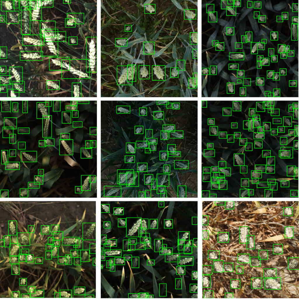
Dataset Format for Comparing KerasCV YOLOv8 Models

The annotations from the original dataset provided in the competition are contained in a train.csv file consisting of 5 column fields:

• image_id: The unique image ID (which is also the filename)
• width: The width of the image
• `height`: The height of the image
• bbox: The bounding box data in [xmin, ymin, width, height] format.
• source: The image source

However, the dataset has been simplified to be used specifically for training in KerasCV. The annotations are converted as XML files for each corresponding image in the [xmin, ymin, xmax, ymax] format. A sample single instance annotation is shown below.

<object>
    <name>wheat_head</name>
    <pose>Unspecified</pose>
    <truncated>0</truncated>
    <difficult>0</difficult>
    <bndbox>
      <xmin>5</xmin>
      <ymin>971</ymin>
      <xmax>54</xmax>
      <ymax>1024</ymax>
    </bndbox>
  </object>

Click here to download the source code to this post

Dataset Preparation for Comparing KerasCV YOLOv8 Models

As usual, we begin by installing the dependencies. Since object detection is being performed, it is imperative to install pycocotools which forms the essence of the COCO evaluation metrics. The latest keras_cv version will also be installed.

!pip install -q pycocotools
!pip install --upgrade git+https://github.com/keras-team/keras-cv -q

Next, the necessary dependencies required for fine-tuning and training will be imported.

import os
import glob
import random
import requests
from zipfile import ZipFile

from dataclasses import dataclass, field
import xml.etree.ElementTree as ET

from tqdm import tqdm
import numpy as np
import cv2

import tensorflow as tf
import keras_cv
from keras_cv import bounding_box

import matplotlib.pyplot as plt

This is followed by setting the required seeds for reproducible results across multiple systems.

def system_config(SEED_VALUE):

    random.seed(SEED_VALUE)
    tf.keras.utils.set_random_seed(SEED_VALUE)

    # Get list of GPUs.
    gpu_devices = tf.config.list_physical_devices('GPU')

    os.environ["CUDA_VISIBLE_DEVICES"] = '0'
    os.environ['TF_CUDNN_DETERMINISTIC'] = '1'

    # Grow the memory usage as the process needs it.
    tf.config.experimental.set_memory_growth(gpu_devices[0], True)

    # Enable using cudNN.
    os.environ['TF_USE_CUDNN'] = "true"

system_config(SEED_VALUE=42)

Downloading and Extracting the Dataset

The data needs to be in the appropriate format before the commencement of the training. The dataset is downloaded and extracted. The download_and_unzip utility specifically performs this task.

# Download and dataset.
def download_and_unzip(url, save_path):

    print("Downloading and extracting assets...", end="")
    file = requests.get(url)
    open(save_path, "wb").write(file.content)

    try:
        # Extract tarfile.
        if save_path.endswith(".zip"):
            with ZipFile(save_path) as zip:
                zip.extractall(os.path.split(save_path)[0])

        print("Done")
    except:
        print("Invalid file")

The data URL for download is specified and extracted once the download is complete.

DATASET_URL = r"https://www.dropbox.com/scl/fi/3gp2mqp1okiyevwnr5pbc/global-wheat-detection.zip?rlkey=kbui4gafys0lok8dqj54li6bj&dl=1"
DATASET_DIR = "global-wheat-detection"
DATASET_ZIP_PATH = os.path.join(os.getcwd(), f"{DATASET_DIR}.zip")

# Download if dataset does not exist.
if not os.path.exists(DATASET_DIR):
    download_and_unzip(DATASET_URL, DATASET_ZIP_PATH)
    os.remove(DATASET_ZIP_PATH)

As mentioned earlier, we will have the annotations as XML files. The following directory structure is maintained.

global-wheat-detection/
├── annotations
│   ├── 0a3cb453f.xml
│   └── ... (3373 files)
├── images
│   ├── 0a3cb453f.jpg
│   └── ... (3373 files)
└── test
   ├── 2fd875eaa.jpg
   └── ... (10 files)

The test data will be used to evaluate the performance of the model when the results are submitted to the competition.

Dataset Configuration for Comparing KerasCV YOLOv8 Models

While the data is being prepared, it also needs to be preprocessed in such a way that it can be fed to the model. We will also apply a few augmentation transformations to enhance the model performance. All the required hyperparameters for the concerned dataset are defined in the DatasetConfig dataclass.

Hyperparameters pertaining to the data, such as the image resolution, the batch size, the images and the annotation paths, the class names, and most importantly, the various augmentation factors such as hue, brightness, translation factors, etc., are handled by this class. The train and validation split (in the ratio 95-5) is also handled here.

@dataclass(frozen=True)
class DatasetConfig:
    DATA_PATH:           str = DATASET_DIR
    IMG_PATH:            str = os.path.join(DATASET_DIR, "images")
    ANN_PATH:            str = os.path.join(DATASET_DIR, "annotations")
    IMAGE_SIZE:        tuple = (832, 832)
    VAL_SPLIT:         float = 0.05
    BATCH_SIZE:          int = 16
    HUE_FACTOR:        float = 0.015
    BRIGHTNESS_FACTOR: float = 0.25
    TRANS_H_FACTOR:    float = 0.1
    TRANS_W_FACTOR:    float = 0.1
    JITTER_RSZ_FACTOR: tuple = (0.8, 1.25)
    CLASSES_DICT:       dict = field(default_factory = lambda:{0 : "wheat_head"})

We will instantiate the DatasetConfig class now.

data_config = DatasetConfig()

The same configuration is maintained across all the models that will be used for fine-tuning.
The image and annotations paths will be shuffled to avoid any unnecessary bias, which will be fed to the tf.data pipeline later on.

IMAGE_PATHS = sorted(glob.glob(os.path.join(data_config.IMG_PATH, "*.jpg")))
ANN_PATHS = sorted(glob.glob(os.path.join(data_config.ANN_PATH, "*.xml")))

# Shuffle the data paths before data preparation.
zipped_data = list(zip(IMAGE_PATHS, ANN_PATHS))
random.shuffle(zipped_data)

IMAGE_PATHS, ANN_PATHS = zip(*zipped_data)
IMAGE_PATHS, ANN_PATHS = list(IMAGE_PATHS), list(ANN_PATHS)

Dataset Preparation using the tf.data API

Next, the XML files will be parsed to extract the bounding box coordinates and the class IDs across each instance.

def parse_annotation(xml_file, data_config = DatasetConfig()):
    tree = ET.parse(xml_file)
    root = tree.getroot()

    class_mapping = data_config.CLASSES_DICT

    bboxes = []
    classes = []
    for obj in root.iter("object"):
        cls = obj.find("name").text

        bbox = obj.find("bndbox")
        xmin = float(bbox.find("xmin").text)
        ymin = float(bbox.find("ymin").text)
        xmax = float(bbox.find("xmax").text)
        ymax = float(bbox.find("ymax").text)

        classes.append(cls)
        bboxes.append([xmin, ymin, xmax, ymax])

    class_ids = [
        list(class_mapping.keys())[list(class_mapping.values()).index(cls)]
        for cls in classes
    ]
    return bboxes, class_ids

Separate lists will be maintained to store the extracted bounding box coordinates and the class IDs after parsing each annotation file.

ALL_BBOX_COORDS = []
ALL_CLASS_IDS = []

for xml_file in tqdm(ANN_PATHS):
    boxes, class_ids = parse_annotation(xml_file)
    ALL_BBOX_COORDS.append(boxes)
    ALL_CLASS_IDS.append(class_ids)

Observe that in object detection, each image can have multiple instances. Hence these lists have to be converted to ragged tensors to handle the variability in object instances.

image_path_tensors  = tf.ragged.constant(IMAGE_PATHS)
bbox_coords_tensors = tf.ragged.constant(ALL_BBOX_COORDS)
class_id_tensors    = tf.ragged.constant(ALL_CLASS_IDS)

Now we will create tensor slices by combing the image paths, the bounding box annotations, and the class IDs to form a Tensorflow dataset. This is achieved using the tf.data.Dataset.from_tensor_slices utility.

data = tf.data.Dataset.from_tensor_slices((image_path_tensors,
                                           bbox_coords_tensors,
                                           class_id_tensors))

Finally, the train and validation splits will be created using the 95-5 ratio.

NUM_VAL = int(len(ANN_PATHS) * data_config.VAL_SPLIT)

# Split the dataset into train and validation sets
train_data = data.skip(NUM_VAL)
val_data = data.take(NUM_VAL)

Data Preprocessing for Training and Validation Data for Comparing KerasCV YOLOv8 Models

The image resolution across all the images in the dataset is (1024, 1024). We will use JiiteredResize for scaling training data with scale distortion, where the image width and height are scaled according to a randomly sampled scaling factor. A cropped version of this scaled image is then padded to the target size. This can serve as an efficient data augmentation pipeline in object detection.

However, using JiiteredResize should be avoided for the validation data. Hence, the validation data should be resized to the target size without cropping or padding.

The load_resize_image function reads and loads the image from the given path and then resizes it based on the resize_image flag.

def load_resize_image(
    image_path,
    resize_image=False,
    size=data_config.IMAGE_SIZE):

    image = tf.io.read_file(image_path)
    image = tf.io.decode_image(image, channels=3)
    image.set_shape([None, None, 3])

    og_image_shape = tf.shape(image)[:2]

    if resize_image:
        image = tf.image.resize(images=image, size=size, method = "bicubic")
        image = tf.cast(tf.clip_by_value(image, 0., 255.), tf.float32)
    else:
        image = tf.cast(image, tf.float32)

    return image, og_image_shape

The bounding boxes should also be resized if their corresponding images are resized. The box_resize function is used to resize and scale the bounding box coordinates based on the target size.

def box_resize(bbox_coords, im_shape, resize=data_config.IMAGE_SIZE):

    resize_wh = list(resize[::-1])
    ratio_wh  = resize_wh / im_shape
    ratio_multipler = tf.cast(tf.concat([ratio_wh, ratio_wh], axis=-1), tf.float32)

    bbox_resize = bbox_coords * ratio_multipler
    bbox_resize = tf.clip_by_value(bbox_resize,
                                   clip_value_min=[0., 0., 0., 0.],
                                   clip_value_max=resize_wh+resize_wh
                                  )
    return bbox_resize

Now that we have created tensor slices using the image paths, bounding box coordinates, and class IDs, it is time to load the corresponding images and perform the appropriate preprocessing. The load_dataset function is used to load the images to disk and preprocess them and their corresponding annotations using the functions described above. 

Bounding boxes and their corresponding target labels in KerasCV need to be coupled to a dictionary having “classes” and “boxes” as the keys. Once the data is pre-processed, the appropriate dictionary will be returned.

def load_dataset(image_path, bbox_coords, class_ids, resize_data=False):
    # Read Image
    image, og_im_shape = load_resize_image(image_path, resize_image=resize_data)
    bbox_tensor = bbox_coords.to_tensor()

    if resize_data:
        bbox_tensor = box_resize(bbox_tensor, og_im_shape)

    bounding_boxes = {
        "classes": tf.cast(class_ids, dtype=tf.float32),
        "boxes": bbox_tensor,
    }
    return {"images": tf.cast(image, tf.float32),
            "bounding_boxes": bounding_boxes}

The images and the bounding boxes will need to be unpacked to visualize the ground truth annotations or the model predictions during inference. The dict_to_tuple utility unpacks the input images and the annotations.

def dict_to_tuple(inputs):
    return inputs["images"], inputs["bounding_boxes"]

Check out the introductory article where we introduced KerasCV and fine-tuned YOLOv8 on a custom dataset.

Data Augmentation and Final Data Preparation for Comparing KerasCV YOLOv8 Models

The following transforms as augmentations will be used:

• Random Translation
• Random Hue
• Random Brightness
• Horizontal Flip
• Jittered Resize

However, for the validation data, no transformations will be used. The images and their corresponding ground truth annotations are resized during data loading itself.

augmenter = tf.keras.Sequential(
            layers=[

                keras_cv.layers.RandomTranslation(
                    height_factor=data_config.TRANS_H_FACTOR,
                    width_factor=data_config.TRANS_W_FACTOR,
                    bounding_box_format="xyxy"),

                keras_cv.layers.RandomHue(factor=data_config.HUE_FACTOR,
                                         value_range=(0., 255.)),
                keras_cv.layers.RandomBrightness(factor=data_config.BRIGHTNESS_FACTOR,
                                                value_range=(0., 255.)),
                keras_cv.layers.RandomFlip(mode="horizontal", bounding_box_format="xyxy"),
                keras_cv.layers.JitteredResize(
                    target_size=data_config.IMAGE_SIZE,
                    scale_factor=data_config.JITTER_RSZ_FACTOR,
                    bounding_box_format="xyxy"
                ),
            ],
            name="Augment_Layer"
)

Finally, we will create batches for both the training and validation data. Furthermore, the training data will be mapped to the augmenter layer defined above.

train_dataset = train_data.map(load_dataset, num_parallel_calls=tf.data.AUTOTUNE)
train_dataset = train_dataset.shuffle(data_config.BATCH_SIZE * 2)
train_dataset = train_dataset.map(augmenter, num_parallel_calls=tf.data.AUTOTUNE)
train_dataset = train_dataset.ragged_batch(data_config.BATCH_SIZE, drop_remainder=False)

train_dataset = train_dataset.map(dict_to_tuple, num_parallel_calls=tf.data.AUTOTUNE)
train_dataset = train_dataset.prefetch(tf.data.AUTOTUNE)

The validation will be resized during load time.

valid_dataset = val_data.map(lambda pths,box, cls: load_dataset(pths,box,cls,resize_data=True),
                             num_parallel_calls=tf.data.AUTOTUNE)
valid_dataset = valid_dataset.ragged_batch(data_config.BATCH_SIZE, drop_remainder=False)

valid_dataset = valid_dataset.map(dict_to_tuple, num_parallel_calls=tf.data.AUTOTUNE)
valid_dataset = valid_dataset.prefetch(tf.data.AUTOTUNE)

Ground Truth Visualizations for Comparing KerasCV YOLOv8 Models

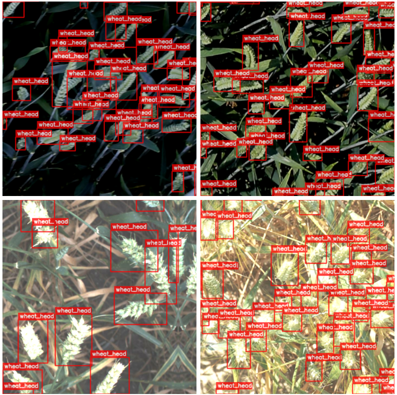
Now that the training and validation data are created, we might want to visualize a few data samples, especially the augmented training data.

The draw_bbox utility accepts the images, bounding box coordinates, class IDs, and confidence scores (available during inference) and plots the corresponding ground truth annotations (or the model predictions).

def draw_bbox(
    image,
    boxes,
    classes,
    scores=None,
    color=(255, 0, 0),
    thickness=-1):

    overlay = image.copy()

    # Reference:
    # https://github.com/Deci-AI/super-gradients/blob/master/src/super_gradients/training/utils/visualization/detection.py

    font_size = 0.25 + 0.07 * min(overlay.shape[:2]) / 100
    font_size = max(font_size, 0.5)
    font_size = min(font_size, 0.8)
    text_offset = 7

    for idx, (box, cls) in enumerate(zip(boxes, classes)):
        xmin, ymin, xmax, ymax = box[0], box[1], box[2], box[3]

        overlay = cv2.rectangle(overlay, (xmin, ymin), (xmax, ymax), color, thickness)

        display_text = f"{data_config.CLASSES_DICT[cls]}"

        if scores is not None:
            display_text+= f": {scores[idx]:.2f}"

        (text_width, text_height), _ = cv2.getTextSize(display_text, cv2.FONT_HERSHEY_SIMPLEX, font_size, 2)

        cv2.rectangle(overlay,
                      (xmin, ymin),
                      (xmin + text_width + text_offset, ymin - text_height - int(15 * font_size)),
                      color, thickness=-1)


        overlay = cv2.putText(
                    overlay,
                    display_text,
                    (xmin + text_offset, ymin - int(10 * font_size)),
                    cv2.FONT_HERSHEY_SIMPLEX,
                    font_size,
                    (255, 255, 255),
                    2, lineType=cv2.LINE_AA,
                )

    return cv2.addWeighted(overlay, 0.75, image, 0.25, 0)

The plot below shows a few samples from the training data.

Comparing KerasCV YOLOv8 Models Creation

As discussed earlier, the following three detection models for YOLOv8 will be dealt with:

• YOLOv8 small
• YOLOv8 medium
• YOLOv8 large

KerasCV provides the pre-trained backbone on MS-COCO; however, the detector heads are initialized with random weights.
The code snippet below creates the YOLOv8 small model having around 13M parameters vindicated from the model preceding it. The corresponding pre-trained backbone preset for the small model is “yolo_v8_s_backbone_coco”.

backbone = keras_cv.models.YOLOV8Backbone.from_preset(
            train_config.BACKBONE, load_weights=True)

yolo = keras_cv.models.YOLOV8Detector(
    num_classes=len(data_config.CLASSES_DICT),
    bounding_box_format="xyxy",
    backbone=backbone,
    fpn_depth=2,
)

print(yolo.summary())

The YOLOv8 medium model is created in a similar fashion; wherein its corresponding backbone preset becomes “yolo_v8_m_backbone_coco”. It has approximately 26M parameters.

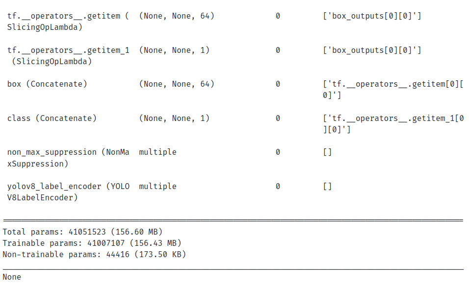
The YOLOv8 large is created with the backbone preset as “yolo_v8_l_backbone_coco”. However, for large and extra-large models, KerasCV recommends specifying fpn_depth for the detector model to be set to 3. The v8 large model has approximately 41M parameters, as can be seen from the model summary.

backbone = keras_cv.models.YOLOV8Backbone.from_preset(
            train_config.BACKBONE, load_weights=True)

yolo = keras_cv.models.YOLOV8Detector(
    num_classes=len(data_config.CLASSES_DICT),
    bounding_box_format="xyxy",
    backbone=backbone,
    fpn_depth=3,
)

print(yolo.summary())

Training Configuration and Model Callbacks for KerasCV YOLOv8

Training Hyperparameters

The training hyper-parameters, such as model backbone, the number of epochs, learning rate, weight decay, etc., are handled by the TrainingConfig class.

@dataclass(frozen=True)
class TrainingConfig:
    BACKBONE:  str = "yolo_v8_s_backbone_coco"
    EPOCHS:    int = 50
    INIT_LR: float = 2e-3
    FINAL_LR:float = 1e-2
    DECAY:   float = 5e-4
    CKPT_DIR:  str = os.path.join("checkpoints_"+"_".join(BACKBONE.split("_")[:3]),
                                  "_".join(BACKBONE.split("_")[:3])+".h5")
    LOGS_DIR:  str = "logs_"+"_".join(BACKBONE.split("_")[:3])

We instantiate the TrainingConfig class below.

train_config = TrainingConfig()

Learning Rate Scheduler for Fine-Tuning KerasCV YOLOv8

The learning rate scheduler updates the learning after each epoch. We will use a linear scheduling algorithm as the learning rate scheduling callback. It is inspired by the LR scheduler from the popular Ultralytics YOLOv8 repository.

def scheduler(epoch, lr):
    return train_config.INIT_LR*(tf.multiply((1 - epoch / train_config.EPOCHS),
                                             (1.0 - train_config.FINAL_LR))
                                 + train_config.FINAL_LR)

Tensorboard Callbacks for Comparing KerasCV YOLOv8 Models

We will also use Tensorboard as callbacks for logging the metrics and losses. The get_callbacks utility defines the LR scheduler and Tensorboard callbacks for logging at the end of every epoch.

def get_callbacks(train_config):

    scheduler_callback = tf.keras.callbacks.LearningRateScheduler(scheduler)

    # Initialize tensorboard callback for logging.
    tensorboard_callback = tf.keras.callbacks.TensorBoard(
        log_dir=train_config.LOGS_DIR,
        histogram_freq=20,
        write_graph=False,
        update_freq="epoch",
    )

    return scheduler_callback, tensorboard_callback

Evaluation Metrics Callback for Comparing KerasCV YOLOv8 Models

In object detection, the performance of the model is interpreted using the Mean Average Precision (mAP) evaluation metric. KerasCV internally computes the metrics using the official pycocotools package through its BoxCOCOMetrics class. The evaluation is performed on the validation data at the end of every epoch.

We will create a custom callback class: EvaluateCOCOMetricsCallback to compute mAP on the validation data at every epoch. Consequently, the model based on the best validation mAP will be saved.

class EvaluateCOCOMetricsCallback(tf.keras.callbacks.Callback):
    def __init__(self, data, save_path):
        super().__init__()
        self.data = data
        self.metrics = keras_cv.metrics.BoxCOCOMetrics(
            bounding_box_format="xyxy",
            evaluate_freq=1e9,
        )

        self.save_path = save_path
        self._options = tf.train.CheckpointOptions()
        self.best_map = -1.0
        self.ckpt_dir = save_path.split("/")[0]
        os.makedirs(self.ckpt_dir, exist_ok=True)

    def on_epoch_end(self, epoch, logs):
        self.metrics.reset_state()
        for i, batch in enumerate(self.data):
            images, y_true = batch[0], batch[1]
            y_pred = self.model.predict(images, verbose=0)
            y_pred_ragged = bounding_box.to_ragged(y_pred)

            self.metrics.update_state(y_true, y_pred_ragged)

        metrics = self.metrics.result(force=True)
        logs.update(metrics)

        current_map = metrics["MaP"]
        # Save the model when mAP improves
        if current_map > self.best_map:
            tf.print(f"\nmAP Improved. Saving model...")
            self.best_map = current_map
            self.model.save_weights(self.save_path, overwrite=True, options=self._options) 

        return logs

Model Compilation for Comparing KerasCV YOLOv8 Models

The Adam optimizer with weight decay defined in the TrainingConfig the class will be used. The model will be compiled with the optimizer, the classification loss (the binary cross entropy loss), and the regression loss (cIoU abbreviated for complete IoU).

You can learn more about the IoU as a regression loss function through this article.

optimizer = tf.keras.optimizers.Adam(
    learning_rate=train_config.INIT_LR,
    weight_decay=train_config.DECAY
)

Model Training and Fine-tuning for Comparing KerasCV YOLOv8 Models

We will finally proceed with the training using the compiled model, the callbacks, and the configured data.

history = yolo.fit(
    train_dataset,
    validation_data=valid_dataset,
    epochs=train_config.EPOCHS,
    callbacks=[EvaluateCOCOMetricsCallback(valid_dataset, train_config.CKPT_DIR),
               scheduler_callback,
               tb_callback]
)

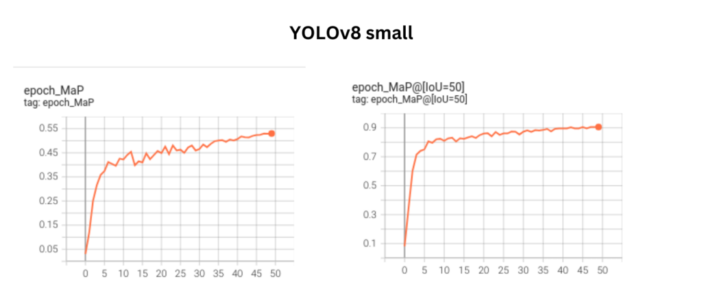
The plot below shows the mAP@0.50-0.95 and mAP@0.5 metric curves for the YOLOv8 small model.

The plot below shows the mAP@0.50-0.95 and mAP@0.5 metric curves for the YOLOv8 medium model.

The plot below shows the mAP@0.50-0.95 and mAP@0.5 metric curves for the YOLOv8 large model.

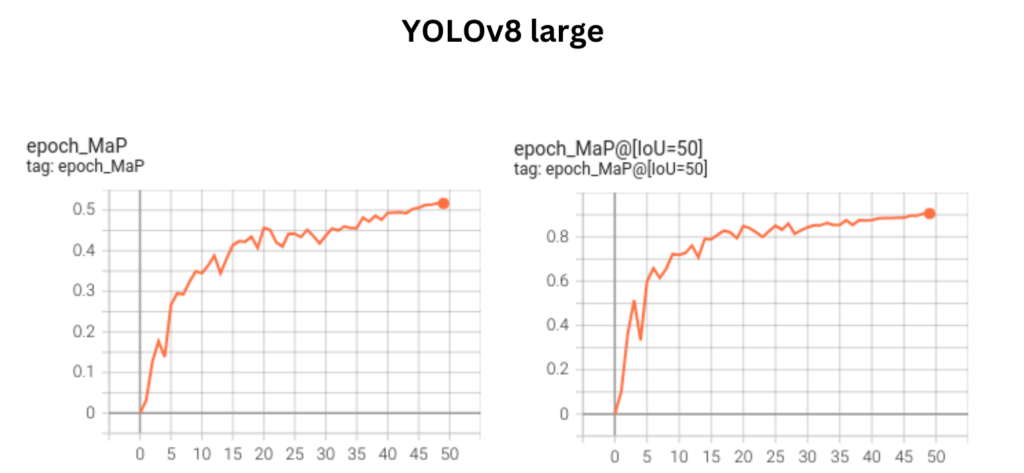
The plots above show the metrics to be in an upward-trending fashion. This indicates that the metrics can be further improved by training the model for more epochs.

The best metrics across each of these models are provided below:

• YOLOv8 small: mAP@0.5-0.95 –> 0.5299 , mAP@0.5 –> 0.9056

• YOLOv8 medium: mAP@0.5-0.95 –>  0.5240, mAP@0.5 –> 0.9033

• YOLOv8 large: mAP@0.5-0.95 –> 0.5168 , mAP@0.5 –> 0.9049

Although the metrics for YOLOv8 small is slightly higher compared to the other two, there is no significant difference in the visualization results across the models.

We have also shared the Tensorboard logs across each of the models so that you can take a closer look.

Predictions Visualization across KerasCV YOLOv8 Models

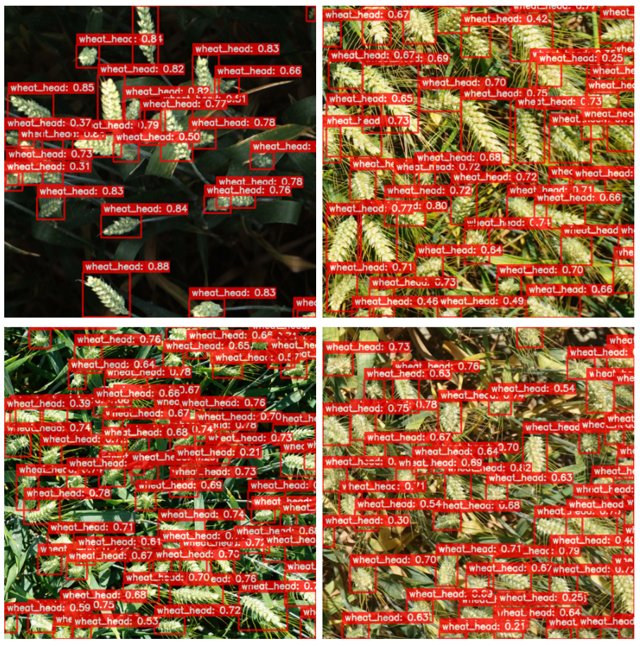
The plot below shows the predictions for the YOLOv8 small model.

The figure below shows the predictions for the YOLOv8 medium model.

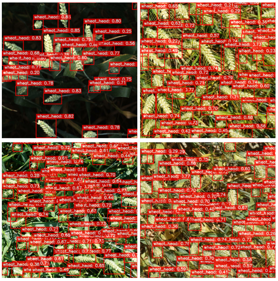
The figure below shows the predictions from the YOLOv8 large model.

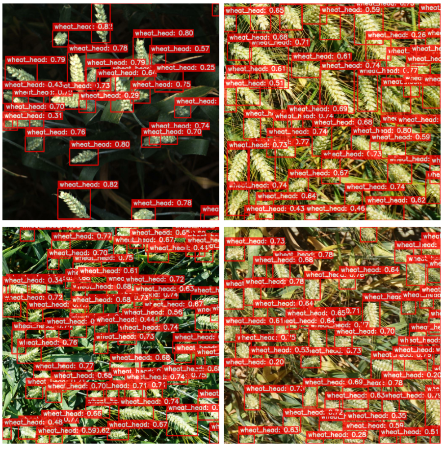
Although the predictions from YOLOv8 small have a slightly better fit across the model instances, the results are not significant enough.

Weighted Boxes Fusion and Comparing KerasCV YOLOv8 Models

Let us look at the Kaggle private and public leaderboard metric scores (in that order) across each of the models that have been trained above.

We have set the IoU (Intersection over Union) and the confidence thresholds for Non-Maximum suppression (as the post-processing step) across each of the models to 0.40 and 0.25, respectively.

The figure below shows the scores for the YOLOv8s model.

The figure below shows the scores for the YOLOv8s model.

The figure below shows the scores for the YOLOv8_l model.

As vindicated from the metrics curve discussed earlier, the scores are in accordance with the v8 small model being the highest, followed by the medium model, and lastly, the large model.

Now that the models are trained separately, the aim is to improve the Kaggle score by ensembling the predictions across these models. This will incorporate a very popular approach called Weighted Boxes Fusion (WBF) that aims to provide unified averaged predictions across multiple models efficiently.

We will use the ensemble-boxes package to apply Weighted Boxes Fusion. Leveraging WBF across multiple models has already been discussed in detail in the Weighted Boxes Fusion in Object Detection: A Comparison with Non-Maximum Suppression article. There are succinct changes complying with the pre-processing step exclusive to Keras.

These models discussed earlier will be used for ensembling the predictions.

We will display a few interesting results by comparing the predictions from the test data between the small model and the ones obtained from WBF side by side.

Let us take a look at the first example inference.

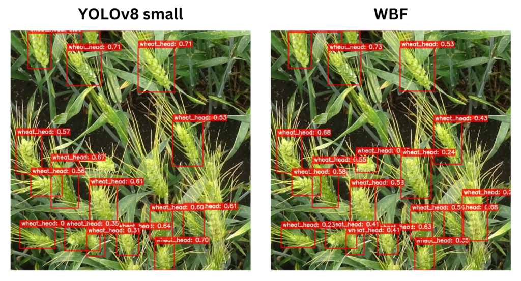
Observe the predictions for the wheat head at the bottom right corner of the image. The WBF approach was able to detect the instance correctly!

Here is another example result.

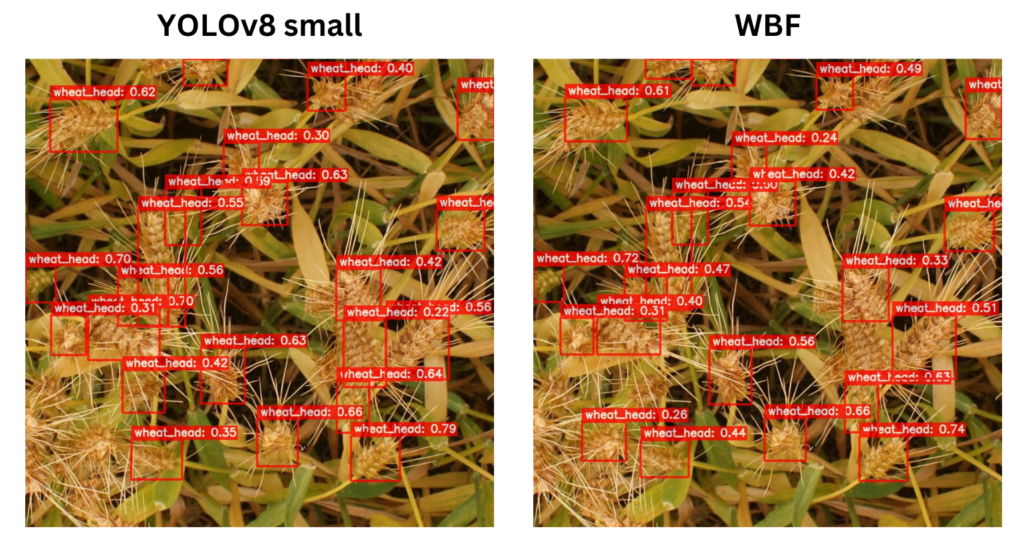
If you can closely observe the wheat head at the bottom left corner of the image, WBF was able to produce an additional detection.

Consequently, the approach using WBF yielded the highest confidence scores, as shown below.

Summary and Conclusion

This wraps up our article. We started by exploring the popular Global Wheat Data and prepared it in accordance with the KerasCV object detection pipeline. Next, we fine-tuned it using the three YOLOv8 detection models, namely V8_small, v8_medium, and v8_large. We also compared the metrics across these models, and it turned out that the v8_small model yielded the highest mAP among the three. The same was reflected in the Kaggle submission scores.

Finally, we applied a more efficient and robust technique called Weighted Boxes Fusion (WBF) as a means of ensembling the predictions to obtain unified “averaged” predictions, which yielded the highest submission score.

We hope that you found this article exciting and insightful. Do let us know in the comments if you have questions!

References

1. Efficient Object Detection with YOLOV8 and KerasCV
2. YOLOv8 MS-COCO Pre-trained Backbones
3. Kaggle Global Wheat Detection Challenge 2020
4. KerasCV Augmentation Layers