Hough Transform with OpenCV (C++/Python)

In this post, we will learn how to detect lines and circles in an image, with the help of a technique called Hough transform.

What is Hough transform?

Hough transform is a feature extraction method for detecting simple shapes such as circles, lines etc in an image.

A “simple” shape is one that can be represented by only a few parameters. For example, a line can be represented by two parameters (slope, intercept) and a circle has three parameters — the coordinates of the center and the radius (x, y, r). Hough transform does an excellent job in finding such shapes in an image.

The main advantage of using the Hough transform is that it is insensitive to occlusion.

Let’s see how Hough transform works by way of an example.

Hough transform to detect lines in an image

100K+ Learners
3 Hours of Learning

Join Free OpenCV Bootcamp

15K+ Learners
3 Hours of Learning

Join Free TensorFlow Bootcamp

10K+ Learners
8 Hours of Learning

Join Free PyTorch Bootcamp

View all AI Free Courses

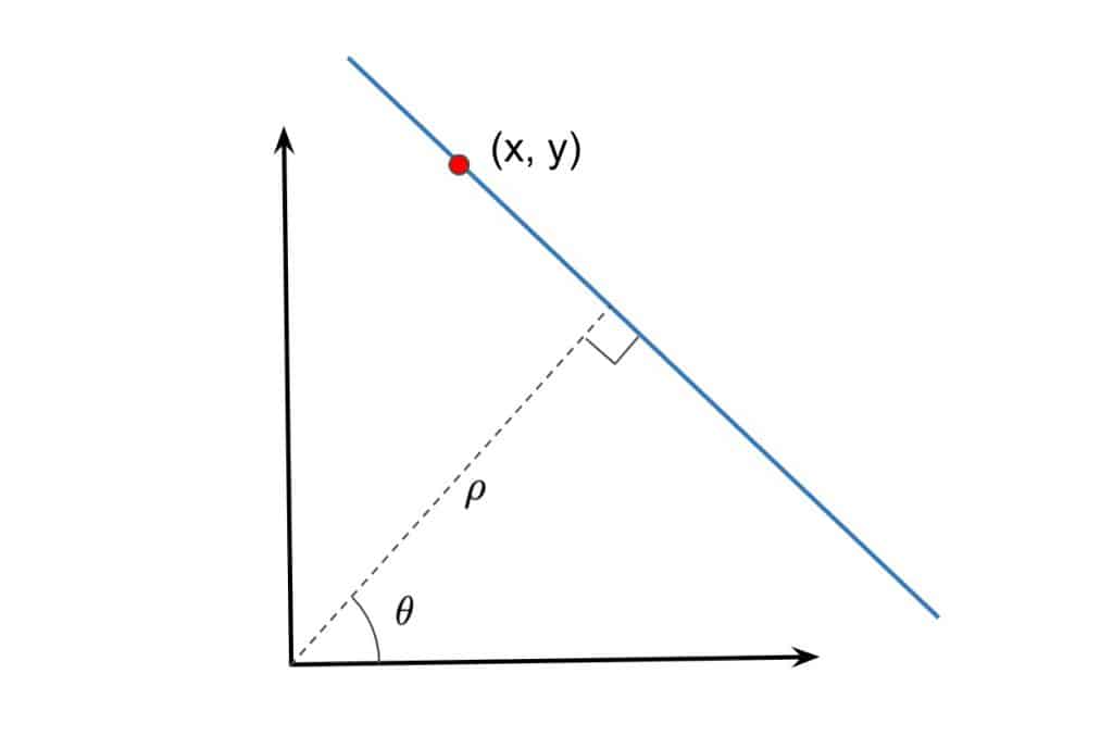
Equation of a line in polar coordinates

From high school math class we know the polar form of a line is represented as:

(1)  

Here represents the perpendicular distance of the line from the origin in pixels, and is the angle measured in radians, which the line makes with the origin as shown in the figure above.

You may be tempted to ask why we did not use the familiar equation of the line given below

The reason is that the slope, m, can take values between – to +. For the Hough transform, the parameters need to be bounded.

You may also have a follow-up question. In the form, is bounded, but can’t take a value between 0 to + ? That may be true in theory, but in practice, is also bounded because the image itself is finite.

Accumulator

When we say that a line in 2D space is parameterized by and , it means that if we any pick a , it corresponds to a line.

Imagine a 2D array where the x-axis has all possible values and the y-axis has all possible values. Any bin in this 2D array corresponds to one line.

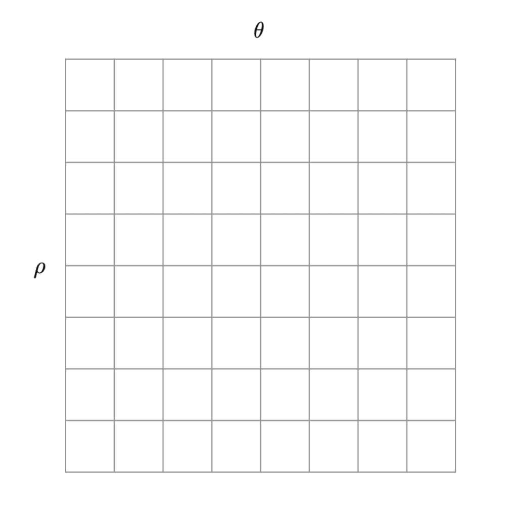
This 2D array is called an accumulator because we will use the bins of this array to collect evidence about which lines exist in the image. The top left cell corresponds to a (-R, 0) and the bottom right corresponds to (R, ).

We will see in a moment that the value inside the bin (, ) will increase as more evidence is gathered about the presence of a line with parameters and .

The following steps are performed to detect lines in an image.

Step 1 : Initialize Accumulator

First, we need to create an accumulator array. The number of cells you choose to have is a design decision. Let’s say you chose a 10×10 accumulator. It means that can take only 10 distinct values and the can take 10 distinct values, and therefore you will be able to detect 100 different kinds of lines. The size of the accumulator will also depend on the resolution of the image. But if you are just starting, don’t worry about getting it perfectly right. Pick a number like 20×20 and see what results you get.

Step 2: Detect Edges

Now that we have set up the accumulator, we want to collect evidence for every cell of the accumulator because every cell of the accumulator corresponds to one line.

How do we collect evidence?

The idea is that if there is a visible line in the image, an edge detector should fire at the boundaries of the line. These edge pixels provide evidence for the presence of a line.

The output of edge detection is an array of edge pixels

Step 3: Voting by Edge Pixels

For every edge pixel (x, y) in the above array, we vary the values of from 0 to and plug it in equation 1 to obtain a value for .

In the Figure below we vary the for three pixels ( represented by the three colored curves ), and obtain the values for using equation 1.

As you can see, these curves intersect at a point indicating that a line with parameters and is passing through them.

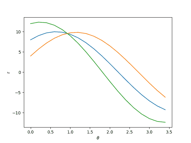
Typically, we have hundreds of edge pixels and the accumulator is used to find the intersection of all the curves generated by the edge pixels.

Let’s see how this is done.

Let’s say our accumulator is 20×20 in size. So, there are 20 distinct values of and so for every edge pixel (x, y), we can calculate 20 (, ) pairs by using equation 1. The bin of the accumulator corresponding to these 20 values of is incremented.

We do this for every edge pixel and now we have an accumulator that has all the evidence about all possible lines in the image.

We can simply select the bins in the accumulator above a certain threshold to find the lines in the image. If the threshold is higher, you will find fewer strong lines, and if it is lower, you will find a large number of lines including some weak ones.

HoughLine: How to Detect Lines using OpenCV

In OpenCV, line detection using Hough Transform is implemented in the function HoughLines and HoughLinesP [Probabilistic Hough Transform]. This function takes the following arguments:

• edges: Output of the edge detector.
• lines: A vector to store the coordinates of the start and end of the line.
• rho: The resolution parameter in pixels.
• theta: The resolution of the parameter in radians.
• threshold: The minimum number of intersecting points to detect a line.

Click here to download the source code to this post

Python:

# Read image 
img = cv2.imread('lanes.jpg', cv2.IMREAD_COLOR) # road.png is the filename
# Convert the image to gray-scale
gray = cv2.cvtColor(img, cv2.COLOR_BGR2GRAY)
# Find the edges in the image using canny detector
edges = cv2.Canny(gray, 50, 200)
# Detect points that form a line
lines = cv2.HoughLinesP(edges, 1, np.pi/180, max_slider, minLineLength=10, maxLineGap=250)
# Draw lines on the image
for line in lines:
    x1, y1, x2, y2 = line[0]
    cv2.line(img, (x1, y1), (x2, y2), (255, 0, 0), 3)
# Show result
cv2.imshow("Result Image", img)

C++:

// Read the image as gray-scale
Mat img = imread('lanes.jpg', IMREAD_COLOR);
// Convert to gray-scale
Mat gray = cvtColor(img, COLOR_BGR2GRAY);
// Store the edges 
Mat edges;
// Find the edges in the image using canny detector
Canny(gray, edges, 50, 200);
// Create a vector to store lines of the image
vector<Vec4i> lines;
// Apply Hough Transform
HoughLinesP(edges, lines, 1, CV_PI/180, thresh, 10, 250);
// Draw lines on the image
for (size_t i=0; i<lines.size(); i++) {
    Vec4i l = lines[i];
    line(src, Point(l[0], l[1]), Point(l[2], l[3]), Scalar(255, 0, 0), 3, LINE_AA);
}
// Show result image
imshow("Result Image", img);

Line Detection Result

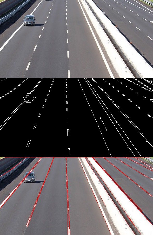
Below we show a result of using hough transform for line detection. Bear in mind the quality of detected lines depends heavily on the quality of the edge map. Therefore, in the real world Hough transform is used when you can control the environment and therefore obtain consistent edge maps or when you can train an edge detector for the specific kind of edges you are looking for.

HoughCircles : Detect circles in an image with OpenCV

In the case of line Hough transform, we required two parameters, (, ) but to detect circles, we require three parameters

• coordinates of the center of the circle.
• radius.

As you can imagine, a circle detector will require a 3D accumulator — one for each parameter.

The equation of a circle is given by

(2)  

The following steps are followed to detect circles in an image: –

1. Find the edges in the given image with the help of edge detectors (Canny).
2. For detecting circles in an image, we set a threshold for the maximum and minimum value of the radius.
3. Evidence is collected in a 3D accumulator array for the presence of circles with different centers and radii.

The function HoughCircles is used in OpenCV to detect the circles in an image. It takes the following parameters:

• image: The input image.
• method: Detection method.
• dp: the Inverse ratio of accumulator resolution and image resolution.
• mindst: minimum distance between centers od detected circles.
• param_1 and param_2: These are method specific parameters.
• min_Radius: minimum radius of the circle to be detected.
• max_Radius: maximum radius to be detected.

Python:

# Read image as gray-scale
img = cv2.imread('circles.png', cv2.IMREAD_COLOR)
# Convert to gray-scale
gray = cv2.cvtColor(img, cv2.COLOR_BGR2GRAY)
# Blur the image to reduce noise
img_blur = cv2.medianBlur(gray, 5)
# Apply hough transform on the image
circles = cv2.HoughCircles(img_blur, cv2.HOUGH_GRADIENT, 1, img.shape[0]/64, param1=200, param2=10, minRadius=5, maxRadius=30)
# Draw detected circles
if circles is not None:
    circles = np.uint16(np.around(circles))
    for i in circles[0, :]:
        # Draw outer circle
        cv2.circle(img, (i[0], i[1]), i[2], (0, 255, 0), 2)
        # Draw inner circle
        cv2.circle(img, (i[0], i[1]), 2, (0, 0, 255), 3)

C++:

// Read the image as gray-scale
img = imread("circles.png", IMREAD_COLOR);
// Convert to gray-scale
gray = cvtColor(img, COLOR_BGR2GRAY);
// Blur the image to reduce noise 
Mat img_blur;
medianBlur(gray, img_blur, 5);
// Create a vector for detected circles
vector<Vec3f>  circles;
// Apply Hough Transform
HoughCircles(img_blur, circles, HOUGH_GRADIENT, 1, img.rows/64, 200, 10, 5, 30);
// Draw detected circles
for(size_t i=0; i<circles.size(); i++) {
    Point center(cvRound(circles[i][0]), cvRound(circles[i][1]));
    int radius = cvRound(circles[i][2]);
    circle(img, center, radius, Scalar(255, 255, 255), 2, 8, 0);
}

HoughCircles function has inbuilt canny detection, therefore it is not required to detect edges explicitly in it.

Circle Detection Result

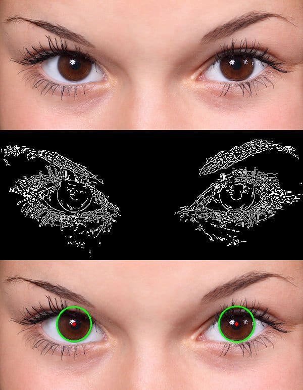
The result of circle detection using Hough transform is shown below. The quality of result depends heavily on the quality of edges you can find, and also on how much prior knowledge you have about the size of the circle you want to detect.