
MASt3R-SLAM is a truly plug and play monocular dense SLAM pipeline that operates in-the-wild. It is first of its kind real-time SLAM system that leverages MASt3R’s 3D Reconstruction priors to achieve superior reconstruction quality while maintaining consistent camera pose tracking. MASt3R-SLAM achieves state-of-the-art results and is even outperforming the widely used ORB-SLAM iterations and DROID-SLAM. It operates real-time with compelling speed of 15FPS on RTX4090.

In this article we will understand the MASt3R-SLAM pipeline with paper explanation and impressive inference results.
- Revising SLAM Concepts
- MASt3R-SLAM: Modern Dense SLAM Method
- Internal Workings of MAST3R-SLAM
- Code Walkthrough of MASt3R-SLAM Inference
- Strengths of MASt3R-SLAM
- Conclusion
- References
If you’re someone just getting started with 3D computer vision, our series of articles will guide through the fundamentals of 3D Vision and Reconstruction.
- 3D Reconstruction with Gaussian Splatting and NeRF
- Stereo and Monocular Depth Estimation
- Understanding Camera calibration and Geometry.
- Monocular Visual SLAM
- DUSt3R: Dense 3D Reconstruction
- MASt3R and MASt3R-SfM
- VGGT: VGGT: Visual Geometry Grounded Transformer
Refresher to SLAM
Simultaneous Localization and Mapping (SLAM) has been a critical component of robot navigation system for decades. SLAM is a challenging and open problem in robotics and it has evolved quite a lot with the advent of deep learning from earlier heuristic based algorithms from 1986 to state of the art methods with just single camera. SLAM enables to create a map of an unknown environment while simultaneously locating the position of the camera or robot within its environment.
Infact mapping (modelling the environment) and localization are mutually dependent where an agent requires a map to localize itself and pose estimation is required to build a map where both are initially unknown. This is why SLAM is often considered the chicken-and-egg problem in robotics. Apart from robotics, SLAM finds its applications in augmented reality, 3D Reconstruction, drone mapping etc,
A typical SLAM pipeline including frontend and backend algorithms will look as follows:
RGB Camera/Sensors Like LiDAR Input → Feature Matching → Pose Estimation/Tracking →Bundle Adjustment → Loop Closure Detection→ Pose Graph optimization
Robust, accurate and real-time SLAM systems that operate on uncalibrated cameras remains a challenging problem. The input to a SLAM system can come from a single camera (monocular) or a stereo camera setup (more than two camera) or LiDAR. Then, it incrementally build a representation (graph construction) and track camera pose relative to the evolving map.
Limitations of Monocular SLAM:
- Monocular SLAM lacks inherent scale information which causes scale ambiguity. Multiple views are required to accurately determine an object’s size by inferring scene geometry over time to establish cross-view coherence.
- Recovering dense 3D structure from 2D images is ill-posed due to loss of depth information as multiple 3D configurations can explain a single view.
- With only a single view, it is difficult to detect and capture features from texture-less surfaces, which can lead to unreliable feature extraction.
- Without camera calibration or IMU, it is hard to obtain reliable poses.
Map Representations in SLAM
SLAM Maps can be categorized as either sparse or dense. Achieving real-time dense construction with just single camera (monocular) is challenging. Existing real-time monocular SLAM systems uses mostly sparse methods.
- Sparse SLAM methods, such as ORB-SLAM track a handful of discrete, distinctive keypoints. These methods are lightweight, fast and provides accurate camera pose tracking in real time. However, the resulting maps are under modelled (less-detailed). Applications that requires rich scene understanding for immersive AR-VR experience or collision avoidance requires sub-pixel level accurate mapping.
- On the other hand, Dense SLAM approaches estimate per-pixel level accurate features from depth across the entire image. This creates a detailed representation of the environment and predicts accurate camera trajectory. However, Dense SLAM is a inverse problem of large dimensionality (computationally intensive) which limits them to operate real time compared to sparse methods. While Droid-SLAM is promising and robust, it still lacks 3D geometric consistency.
Major SLAM Paradigms
- Filtering Approaches : These methods model the problem as Online State Estimation where the robot state is updated on the go with new measurements based on previous measurements. These methods typically don’t use any explicit loop detection or global optimization methods to refine their poses when the agents revisits previously mapped area or landmark.
Examples: Kalman Filter based EKF SLAM, Particle Filter – FAST SLAM etc.
- Smoothing Approaches: These methods estimate the entire trajectory by optimizing over entire history of measurements. The desirable property is they can refine or adjust their past estimate based on new information mainly during loop closure where separate loop detection or global optimization phase is involved.
Examples: Least Squares Optimization, Pose Graph SLAM, Bundle Adjustment (BA) etc.
MASt3R-SLAM uses the standard Graph Construction and Optimization technique steps very similar to DUSt3R or MASt3R-SfM. If you are someone who have worked with SfM pipelines, you might be familiar with the term Bundle Adjustment. The key difference is BA adjusts both pose and 3D points whereas Pose Graph optimizes only for camera pose.
DUSt3R and MASt3R pioneered SfM from two-view 3D Reconstruction which outputs pointmaps directly in a common coordinate frame solving 3D reconstruction and camera pose estimation tasks in a joint fashion. In a similar way what if we could make sure of these 3D Reconstruction priors for SLAM? This is what MASt3R-SLAM tries to achieve.
MASt3R-SLAM: Modern Dense SLAM Method
For consistent camera tracking in SLAM, the system should have good understanding about varying camera poses over time. MASt3R-SLAM by Riku Murai et al. is the first pipeline to fully integrate a two-view 3D prior into a realtime incremental SLAM system. By leveraging strong 3D priors of MASt3R, it enables descriptor-based retrieval to deliver globally consistent camera poses and detailed dense maps realtime at 15FPS on a single consumer grade GPU like RTX 4090 paired with i9-12th gen.
👉 We have covered MASt3R indepth in the previous article of this series, so be sure to check it out. Here, we will discuss only the high level concepts required so that it all ties together.
MASt3R is a SOTA zero shot foundational 3D reconstruction model trained on large scale datasets with excellent understanding about a 3D scene. MASt3R doesn’t require any camera calibration or known camera poses, making it capable of operating in-the-wild scenarios and is robust to challenging real-world conditions.
![Reconstruction from our dense monocular SLAM system
on the Burghers sequence [55]. Using the two-view predictions
from MASt3R shown on the left, our system achieves globally
consistent poses and geometry in real-time even without a known
camera model.](https://learnopencv.com/wp-content/uploads/2025/04/MASt3R-SLAM-with-two-view-3D-Piror-of-MASt3R-realtime-reconstruction-and-mapping.jpg "MASt3R-SLAM-with-two-view-3D-Piror-of-MASt3R-realtime-reconstruction-and-mapping – LearnOpenCV")
MASt3R takes in a pair of images from different viewpoints and outputs two pointmaps in a shared coordinate frame, aiming accurate pixel matching between these pairs.
For every new frame, MASt3R predicts outputs as:
- Pointmaps
 ,
, 
- Confidence
 ,
, 
- Learned Descriptors/Features
 ,
, 
- Feature Confidences
 ,
, 
It grounds image matching as a 3D task allowing it to solve multiple 3D downstream tasks simultaneously within a single unified framework. As a result, 3D priors of MASt3R is found to be extremely useful in Structure-from-Motion pipelines.


Internal Workings of MAST3R-SLAM
MASt3R-SLAM operates without assuming any known parametric camera (pinhole) model, rather simply it uses a generic central camera model where all light rays pass through a single point for an image by normalising a pointmap into rays. This removes the need for camera calibration yet achieves globally consistent poses and dense geometry in real time.
This enables SLAM with time-varying camera models such as the highly dynamic zooming upto 5x shown below,

shown by two consecutive keyframes for an outdoor scene
Generic Camera Model: Pointmap to Rays
Unlike MASt3R which produces metric scale predictions, the authors reports that using native metric scale of MASt3R across different views can lead to significant error. To address this, scale is preserved across pairwise predictions with a scale factor rather than a global metric scale. So what does this mean? It focuses on relative scale between two views rather than forcing all views to conform to a absolute scale by optimizing all poses as:
T ∈ Sim(3)

where,
 represents transformation or pose of a camera in 3D space
 : Similarity transformation group in three dimensions (Rotation, Translation and Uniform Scaling). A similarity transformation is a geometric transformation which preserves the shape of an object intact but can change its size, position and orientation.
Though MASt3R produces robust predictions, it’s result are not perfect as they may contain noise or poor correlations. Building on top of MASt3R priors, MASt3R SLAM introduces novel technique in its pipeline for matching, fusion and optimization to achieve real-time, low-latency performance and generate global consistent maps. It requires no post-processing or offline computation.
It’s modules include:
1. MASt3R Prediction and Pointmap Matching
2. Front-End Tracking and Local fusion
3. Keyframe Graph Construction and Loop Closure
4. Second-Order Global Optimization
5. Relocalization and Camera Handling
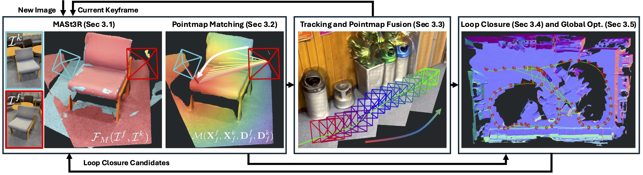
1. MASt3R Prediction and Efficient Pointmap Matching
Given two images, MASt3R finds dense pixel correspondence between two pointmap outputs , . Matching between a query image and all target pairs for every pixel, using naive brute-force search is extremely slow and computationally expensive. To mitigate this MASt3R uses a coarse to fine matching scheme; however it is still slow for dense matching. Therefore, MASt3R-SLAM proposes Iterative Projective Matching (IPM) technique along with feature refinement. By this the system successfully combines strength of learning-based with geometric techniques for robust than using either one.
What is Iterative Projective Matching?
Consider MASt3R’s output: a 3D pointmap  of image
  expressed in the coordinate frame of image
  . Similarly, every pixel in image has a ray (known) shooting out from camera center for all the pixels across the image.
def point_to_ray_dist(X, jacobian=False):
    b = X.shape[:-1]

    d = point_to_dist(X)
    d_inv = 1.0 / d
    r = d_inv * X
    rd = torch.cat((r, d), dim=-1)  # Dim 4
    if not jacobian:
        return rd
    else:
        d_inv_2 = d_inv**2
        I = torch.eye(3, device=X.device, dtype=X.dtype).repeat(*b, 1, 1)
        dr_dX = d_inv.unsqueeze(-1) * (
            I - d_inv_2.unsqueeze(-1) * (X.unsqueeze(-1) @ X.unsqueeze(-2))
        )
        dd_dX = r.unsqueeze(-2)
        drd_dX = torch.cat((dr_dX, dd_dX), dim=-2)
        return rd, drd_dX
The goal is to find which pixel ray (target) is in same direction of the known unit-length ray  . This is found by minimizing the Eucledian distance
(![|\Psi\bigl(X^i_i[p]\bigr) - \Psi(x)|^2](https://learnopencv.com/wp-content/ql-cache/quicklatex.com-0972e85ffef05269728c8e57d84b87f0_l3.png) ),
),
which indirectly minimizes the angular difference  between the ray at
  and corresponding 3D point from image . The process starts with an initial guess for pixel
  ,
,
![\mathbf{p}^* = \arg\min_{\mathbf{p}} \left| \psi\left( \left[ \mathbf{X}^{i}_{i} \right]{\mathbf{p}} \right) - \psi(\mathbf{x}) \right|^2](https://learnopencv.com/wp-content/ql-cache/quicklatex.com-15a64c987f93e45dc5f910eca4c0c68d_l3.png)
where,  is simply the patch pixel whose descriptor has the highest cosine similarity with the query descriptor.

Feature Refinement
With good geometric initialization, coarse pixel matches from IPM, then perform a coarse to fine search in local patch within a  window around matched pixels (feature space
  ). By comparing MASt3R’s learned descriptors of image and image we establish dense correspondence which nails a sub-pixel level accurate matching.
By combining IPM and Feature Refinement, the system provides dense, reliable correspondences and enables massive GPU parallelization scheme converging rapidly within 10 iterations and still remain unbiased by previous pose estimates.
def match(X11, X21, D11, D21, idx_1_to_2_init=None):
    idx_1_to_2, valid_match2 = match_iterative_proj(X11, X21, D11, D21, idx_1_to_2_init)
    return idx_1_to_2, valid_match2


def pixel_to_lin(p1, w):
    idx_1_to_2 = p1[..., 0] + (w * p1[..., 1])
    return idx_1_to_2


def lin_to_pixel(idx_1_to_2, w):
    u = idx_1_to_2 % w
    v = idx_1_to_2 // w
    p = torch.stack((u, v), dim=-1)
    return p


def prep_for_iter_proj(X11, X21, idx_1_to_2_init):
    b, h, w, _ = X11.shape
    device = X11.device

    # Ray image
    rays_img = F.normalize(X11, dim=-1)
    rays_img = rays_img.permute(0, 3, 1, 2)  # (b,c,h,w)
    gx_img, gy_img = img_utils.img_gradient(rays_img)
    rays_with_grad_img = torch.cat((rays_img, gx_img, gy_img), dim=1)
    rays_with_grad_img = rays_with_grad_img.permute(
        0, 2, 3, 1
    ).contiguous()  # (b,h,w,c)

    # 3D points to project
    X21_vec = X21.view(b, -1, 3)
    pts3d_norm = F.normalize(X21_vec, dim=-1)

    # Initial guesses of projections
    if idx_1_to_2_init is None:
        # Reset to identity mapping
        idx_1_to_2_init = torch.arange(h * w, device=device)[None, :].repeat(b, 1)
    p_init = lin_to_pixel(idx_1_to_2_init, w)
    p_init = p_init.float()

    return rays_with_grad_img, pts3d_norm, p_init


def match_iterative_proj(X11, X21, D11, D21, idx_1_to_2_init=None):
    cfg = config["matching"]
    b, h, w = X21.shape[:3]
    device = X11.device

    rays_with_grad_img, pts3d_norm, p_init = prep_for_iter_proj(
        X11, X21, idx_1_to_2_init
    )
    p1, valid_proj2 = mast3r_slam_backends.iter_proj(
        rays_with_grad_img,
        pts3d_norm,
        p_init,
        cfg["max_iter"],
        cfg["lambda_init"],
        cfg["convergence_thresh"],
    )
    p1 = p1.long()

    # Check for occlusion based on distances
    batch_inds = torch.arange(b, device=device)[:, None].repeat(1, h * w)
    dists2 = torch.linalg.norm(
        X11[batch_inds, p1[..., 1], p1[..., 0], :].reshape(b, h, w, 3) - X21, dim=-1
    )
    valid_dists2 = (dists2 < cfg["dist_thresh"]).view(b, -1)
    valid_proj2 = valid_proj2 & valid_dists2

    if cfg["radius"] > 0:
        (p1,) = mast3r_slam_backends.refine_matches(
            D11.half(),
            D21.view(b, h * w, -1).half(),
            p1,
            cfg["radius"],
            cfg["dilation_max"],
        )

    # Convert to linear index
    idx_1_to_2 = pixel_to_lin(p1, w)

    return idx_1_to_2, valid_proj2.unsqueeze(-1)
2. Front-End Tracking and Local Pointmap fusion
For every new frame, MASt3R provides pointmap predictions, that are used for camera pose tracking and local geometry fusion. Each incoming frames pose is tracked relative to existing keyframes of the map. A graph is constructed by maintaining node-edge relationship between matching frame and their relative camera Sim(3) pose  is recovered.
Then geometric information is locally fused into the most recent keyframe’s canonical pointmap  via a weighted running average which incrementally refines both pose and map representation.
Unlike DUSt3R and MASt3R, which uses direct 3D Point error, MASt3R-SLAM uses Ray based error (angular difference between rays) which is more robust,
where,
 is the match confidence weight
- Huber norm
 down weighs outliers.
  def track(self, frame: Frame):
        keyframe = self.keyframes.last_keyframe()

        idx_f2k, valid_match_k, Xff, Cff, Qff, Xkf, Ckf, Qkf = mast3r_match_asymmetric(
            self.model, frame, keyframe, idx_i2j_init=self.idx_f2k
        )
        # Save idx for next
        self.idx_f2k = idx_f2k.clone()

        # Get rid of batch dim
        idx_f2k = idx_f2k[0]
        valid_match_k = valid_match_k[0]

        Qk = torch.sqrt(Qff[idx_f2k] * Qkf)

        # Update keyframe pointmap after registration (need pose)
        frame.update_pointmap(Xff, Cff)

        use_calib = config["use_calib"]
        img_size = frame.img.shape[-2:]
        if use_calib:
            K = keyframe.K
        else:
            K = None

        # Get poses and point correspondneces and confidences
        Xf, Xk, T_WCf, T_WCk, Cf, Ck, meas_k, valid_meas_k = self.get_points_poses(
            frame, keyframe, idx_f2k, img_size, use_calib, K
        )

        # Get valid
        # Use canonical confidence average
        valid_Cf = Cf > self.cfg["C_conf"]
        valid_Ck = Ck > self.cfg["C_conf"]
        valid_Q = Qk > self.cfg["Q_conf"]

        valid_opt = valid_match_k & valid_Cf & valid_Ck & valid_Q
        valid_kf = valid_match_k & valid_Q

        match_frac = valid_opt.sum() / valid_opt.numel()
        if match_frac < self.cfg["min_match_frac"]:
            print(f"Skipped frame {frame.frame_id}")
            return False, [], True

        try:
            # Track
            if not use_calib:
                T_WCf, T_CkCf = self.opt_pose_ray_dist_sim3(
                    Xf, Xk, T_WCf, T_WCk, Qk, valid_opt
                )
            else:
                T_WCf, T_CkCf = self.opt_pose_calib_sim3(
                    Xf,
                    Xk,
                    T_WCf,
                    T_WCk,
                    Qk,
                    valid_opt,
                    meas_k,
                    valid_meas_k,
                    K,
                    img_size,
                )
        except Exception as e:
            print(f"Cholesky failed {frame.frame_id}")
            return False, [], True

        frame.T_WC = T_WCf

        # Use pose to transform points to update keyframe
        Xkk = T_CkCf.act(Xkf)
        keyframe.update_pointmap(Xkk, Ckf)
        # write back the fitered pointmap
        self.keyframes[len(self.keyframes) - 1] = keyframe

        # Keyframe selection
        n_valid = valid_kf.sum()
        match_frac_k = n_valid / valid_kf.numel()
        unique_frac_f = (
            torch.unique(idx_f2k[valid_match_k[:, 0]]).shape[0] / valid_kf.numel()
        )

        new_kf = min(match_frac_k, unique_frac_f) < self.cfg["match_frac_thresh"]

        # Rest idx if new keyframe
        if new_kf:
            self.reset_idx_f2k()

        return (
            new_kf,
            [
                keyframe.X_canon,
                keyframe.get_average_conf(),
                frame.X_canon,
                frame.get_average_conf(),
                Qkf,
                Qff,
            ],
            False,
        )
3. Keyframe Graph Construction and Loop Closure
Key frame selection: Rather than inserting every frame in the pose-graph, a frame is registered as keyframe when tracking quality or geometric overlap falls below a threshold based on correspondence. Each keyframe becomes node in the pose-graph, by adding a sequential edge to the previous keyframe.
Loop Closure via MASt3R Retrieval:
MASt3R-SLAM follows similar design principles of MASt3R-SfM by using MASt3R checkpoint as a retriever between current keyframe and the previous unique keyframes.
After each keyframe  is inserted, per-pixel encodings of MASt3R features and their descriptors are aggregated into a compact codebook using Aggregated Selective Matching Kernel (ASMK). This is similar to the design priniciples of MASt3R-SfM to retrieve candidate descriptors and is extremely fast. If the camera frame revisits a previously mapped area, loop closure is detected and
 top_K visually similar candidate keyframes are retrieved to match the descriptors of the current query keyframe using a simple L2 distance. Post this we perform IPM and feature refinement to count inlier correspondences. If enough reliable matches  are obtained, we add a bidirectional edge
  between those nodes based on retrieval scores above a threshold
  .
.
Filtering has a rich history in SLAM, and yields the benefit of leveraging information from all frames without having to explicitly optimise for all camera poses and store all predicted pointmaps from the decoder in the backend.
Then, incrementally build an image retrieval database using MASt3R features which enables real-time relocalisation and loop closure which corrects the drift for globally consistent poses and dense geometry.
For example,
Database retrieval 3 :  {1}
Database retrieval 4 :  {0, 1}
Database retrieval 5 :  {0}
. . .
Database retrieval 14 :  {2, 3}
Database retrieval 15 :  {2, 3}
Database retrieval 16 :  {1, 2, 13}
4. Second Order Global Optimization – Backend Optimization
Previous methods use first-order optimization, however they need rescaling after every iteration whereas in MASt3R-SLAM, second order optimisation speeds up and achieves global consistency across all camera poses (trajectory) and dense map of the environment or scene. Since gradient descent converges slowly, MASt3R-SLAM leverages Gauss-Newton optimization to achieve efficient large-scale updates.
Ray error for all the edges in the graph.

The below image from the paper, shows that instead of using 3D point error, ray error formulation for uncalibrated tracking and backend optimization has significantly improved the performance across datasets and mitigated the effect of inaccurate pointmap predictions.

def run_backend(cfg, model, states, keyframes, K):
    set_global_config(cfg)

    device = keyframes.device
    factor_graph = FactorGraph(model, keyframes, K, device)
    retrieval_database = load_retriever(model)

    mode = states.get_mode()
    while mode is not Mode.TERMINATED:
        mode = states.get_mode()
        if mode == Mode.INIT or states.is_paused():
            time.sleep(0.01)
            continue
        if mode == Mode.RELOC:
            frame = states.get_frame()
            success = relocalization(frame, keyframes, factor_graph, retrieval_database)
            if success:
                states.set_mode(Mode.TRACKING)
            states.dequeue_reloc()
            continue
        idx = -1
        with states.lock:
            if len(states.global_optimizer_tasks) > 0:
                idx = states.global_optimizer_tasks[0]
        if idx == -1:
            time.sleep(0.01)
            continue

        # Graph Construction
        kf_idx = []
        # k to previous consecutive keyframes
        n_consec = 1
        for j in range(min(n_consec, idx)):
            kf_idx.append(idx - 1 - j)
        frame = keyframes[idx]
        retrieval_inds = retrieval_database.update(
            frame,
            add_after_query=True,
            k=config["retrieval"]["k"],
            min_thresh=config["retrieval"]["min_thresh"],
        )
        kf_idx += retrieval_inds

        lc_inds = set(retrieval_inds)
        lc_inds.discard(idx - 1)
        if len(lc_inds) > 0:
            print("Database retrieval", idx, ": ", lc_inds)

        kf_idx = set(kf_idx)  # Remove duplicates by using set
        kf_idx.discard(idx)  # Remove current kf idx if included
        kf_idx = list(kf_idx)  # convert to list
        frame_idx = [idx] * len(kf_idx)
        if kf_idx:
            factor_graph.add_factors(
                kf_idx, frame_idx, config["local_opt"]["min_match_frac"]
            )

        with states.lock:
            states.edges_ii[:] = factor_graph.ii.cpu().tolist()
            states.edges_jj[:] = factor_graph.jj.cpu().tolist()

        if config["use_calib"]:
            factor_graph.solve_GN_calib()
        else:
            factor_graph.solve_GN_rays()

        with states.lock:
            if len(states.global_optimizer_tasks) > 0:
                idx = states.global_optimizer_tasks.pop(0)
5.1 Relocalization
When camera tracking fails, relocalisation mode starts. Again, for a new frame the previous steps are carried out again to added as a new keyframe into the graph and tracking resumes.
Reasons for Losing Tracking:
- Insufficient matches due to occlusion, fast motion, lack of features, or sudden changes in illumination.
- Outliers – Incorrect or noisy feature correspondence can disrupt accurate pose estimation.
- Degenerate configuration: In certain cases, the scene geometry or camera motions can introduce ambiguities making it difficult to maintain a reliable track.
def relocalization(frame, keyframes, factor_graph, retrieval_database):
    # we are adding and then removing from the keyframe, so we need to be careful.
    # The lock slows viz down but safer this way...
    with keyframes.lock:
        kf_idx = []
        retrieval_inds = retrieval_database.update(
            frame,
            add_after_query=False,
            k=config["retrieval"]["k"],
            min_thresh=config["retrieval"]["min_thresh"],
        )
        kf_idx += retrieval_inds
        successful_loop_closure = False
        if kf_idx:
            keyframes.append(frame)
            n_kf = len(keyframes)
            kf_idx = list(kf_idx)  # convert to list
            frame_idx = [n_kf - 1] * len(kf_idx)
            print("RELOCALIZING against kf ", n_kf - 1, " and ", kf_idx)
            if factor_graph.add_factors(
                frame_idx,
                kf_idx,
                config["reloc"]["min_match_frac"],
                is_reloc=config["reloc"]["strict"],
            ):
                retrieval_database.update(
                    frame,
                    add_after_query=True,
                    k=config["retrieval"]["k"],
                    min_thresh=config["retrieval"]["min_thresh"],
                )
                print("Success! Relocalized")
                successful_loop_closure = True
                keyframes.T_WC[n_kf - 1] = keyframes.T_WC[kf_idx[0]].clone()
            else:
                keyframes.pop_last()
                print("Failed to relocalize")

        if successful_loop_closure:
            if config["use_calib"]:
                factor_graph.solve_GN_calib()
            else:
                factor_graph.solve_GN_rays()
        return successful_loop_closure
5.2 Camera Calibration
Given, known camera intrinsics K, switch residuals from ray error to pixel reprojection error.

With this simple modification, SOTA results is achieved with low ATE on benchmaks like TUm RGB-D and 7 Scenes.

Comparison of MASt3R-SLAM vs DROID-SLAM vs ORB-SLAM
MASt3R-SLAM consistently outperforms or on-par with other baselines on camera pose and geometry consistency like ORB-SLAM3 and DROID-SLAM across multiple datasets.
The following image clearly shows MASt3R-SLAM produces superior reconstruction quality compared to DRIOID-SLAM with less RMSE Chamfer.


on the ETH3D SLAM benchmark
| Feature/System | MASt3R-SLAM | DROID-SLAM | ORB-SLAM3 |
| Approach | Deep Learning based, utilizing two-view 3D reconstruction priors | Deep Learning based, employing recurrent optimization with dense bundle adjustement | Classifical feature-based SLAM with visual-inertial and multi-map capabilities |
| Sensor Support | Monocular | Monocular,Stereo, RGB-D | Monocular, Stereo, RGB-D, Visual-Inertial (IMU) |
| Mapping Type | Dense | Dense | Sparse |
| Loop Closure and Relocalization | Yes, via ASMK-based feature retrieval and graph optimization | Yes, integrated into its optimization framework | Yes, with improved place recognition and multi-map merging capabilities |
| Real-time | Yes (~15 FPS on RTX4090) | Yes | Yes |
| Benchmark | Outperforms DROID-SLAM and OR-SLAM in extreme conditions; excels in low-light and low-texture scenarios | Excels in medium-difficult scenarios and outperforms MASt3R-SLAM in certain datasets | Demonstrates superior accuracy in visual-inertial configurations and structured outdoor environments like KITTI |

Code Walkthrough of MASt3R-SLAM Inference
To set up locally, follow along the instructions outlined in the README of MASt3R-SLAM Repository.
git clone https://github.com/rmurai0610/MASt3R-SLAM.git --recursive
cd MASt3R-SLAM/

# if you've clone the repo without --recursive run
# git submodule update --init --recursive

pip install -e thirdparty/mast3r
pip install -e thirdparty/in3d
pip install --no-build-isolation -e .


# Optionally install torchcodec for faster mp4 loading
pip install torchcodec==0.1
After cloning download the model under checkpoints folder,
mkdir -p checkpoints/
wget https://download.europe.naverlabs.com/ComputerVision/MASt3R/MASt3R_ViTLarge_BaseDecoder_512_catmlpdpt_metric.pth -P checkpoints/
wget https://download.europe.naverlabs.com/ComputerVision/MASt3R/MASt3R_ViTLarge_BaseDecoder_512_catmlpdpt_metric_retrieval_trainingfree.pth -P checkpoints/
wget https://download.europe.naverlabs.com/ComputerVision/MASt3R/MASt3R_ViTLarge_BaseDecoder_512_catmlpdpt_metric_retrieval_codebook.pkl -P checkpoints/
On RTX 3080Ti the setup achieved around 5-7FPS depending upon the video resolution with a variable VRAM usage between 9-11 GB based on video length.
To run inference on the TUM/freiburg1_room image sequence or other datasets, simply run the corresponding bash scripts .sh,
bash ./scripts/download_tum.sh
python main.py --dataset datasets/tum/rgbd_dataset_freiburg1_room/ --config config/calib.yaml
👉 Note: The pipeline only supports .png image sequences, if your input is in different image format, be sure to check beforehand. Otherwise one may need to modify the dataloader.py script manually to adapt the code to different input types.
Inference 1

Inference 2

Strengths of MASt3R-SLAM
- MASt3R-SLAM assumes no camera specifics, and adapts a simple central camera model where all the rays pass through a centre.
- Operates realtime with compelling speed of 15FPS on RTX4090.
- Achieves state-of-the-art results and is first of its kind real-time SLAM system that leverages MASt3R’s 3D Reconstruction priors to represent accurate geometry and camera tracjectory.
- Robust to rotational motion and low-texture environments.
Conclusion
We see the SLAM results and speed are quite impressive on a consumer grade GPUs like 4090 and 3080Ti. The authors recommends to adapt MASt3R SLAM to distorted lens or extreme lens like 360° or fisheye training MASt3R checkpoint on those specific datasets should help them to accomodate these extreme viewpoint changes and reduce reprojection drift. MASt3R is licensed under CC by NC (non-commercial) which limits its applications into any commercial solutions, however be sure to do your own research about license carefully before integrating this setup.
Hope you find this read interesting. Do let us know your feedback via our social handles.


100K+ Learners
Join Free OpenCV Bootcamp3 Hours of Learning