Conditional GAN (cGAN) in PyTorch and TensorFlow

Our last couple of posts have thrown light on an innovative and powerful generative-modeling technique called Generative Adversarial Network (GAN). Yes, the GAN story started with the vanilla GAN. But no, it did not end with the Deep Convolutional GAN. To take you marching forward here comes the Conditional Generative Adversarial Network also known as Conditional GAN. We not only discussed GAN’s basic intuition, its building blocks (generator and discriminator), and essential loss function. But also went ahead and implemented the vanilla GAN and Deep Convolutional GAN to generate realistic images.

If you followed the previous blog posts closely, you noticed that the GAN is trained in a completely unsupervised and unconditional fashion, meaning no labels are involved in the training process. Though the GAN model can generate new realistic samples for a particular dataset, we have zero control over the type of images generated.

But what if we want our GAN model to generate only shirt images, not random ones containing trousers, coats, sneakers, etc.? For instance, after training the GAN, what if we sample a noise vector from a standard normal distribution, feed it to the generator, and obtain an output image representing any image from the given dataset. It may be a shirt, and it may not be a shirt. Remember, in reality; you have no control over the generation process.

This post is part of the series on Generative Adversarial Networks in PyTorch and TensorFlow, which consists of the following tutorials:

1. Introduction to Generative Adversarial Networks (GANs)
2. Deep Convolutional GAN in PyTorch and TensorFlow
3. Conditional GAN (cGAN) in PyTorch and TensorFlow
4. Pix2Pix: Paired Image-to-Image Translation in PyTorch & TensorFlow

However, if you are bent on generating only a shirt image, you can keep generating examples until you get the shirt image you want. But are you fine with this brute-force method? Take another example- generating human faces. Again, you cannot specifically control what type of face will get produced. No way can you direct the Generator to synthesize pointedly a male or a female face, let alone other features like age or facial expression. So what is the way out?

Try leveraging the conditional version of GAN, called the Conditional Generative Adversarial Network (CGAN). Okay, so let’s get to know this Conditional GAN and especially see how we can control the generation process.

Like last time, we will be giving you a bonus by implementing CGAN, both in PyTorch and TensorFlow, on the Rock Paper Scissors Dataset. Let’s get going!

1. Introduction
2. Purpose of Conditional Generator and Discriminator
3. Coding Conditional GAN
   1. TensorFlow Implementation
   2. PyTorch Implementation
4. Bonus: Class-Conditional Latent Space Interpolation

What is a Conditional GAN?

In 2014, Mehdi Mirza (a Ph.D. student at the University of Montreal) and Simon Osindero (an Architect at Flickr AI), published the Conditional Generative Adversarial Nets paper, in which the generator and discriminator of the original GAN model are conditioned during the training on external information. This information could be a class label or data from other modalities. Here, we will use class labels as an example. This paper has gathered more than 4200 citations so far!

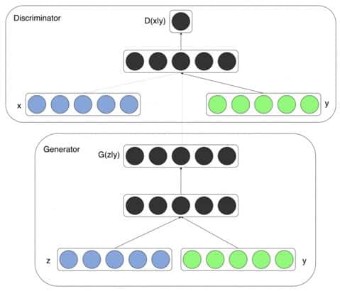
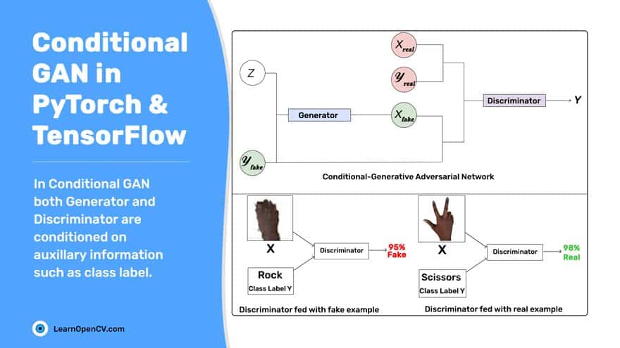
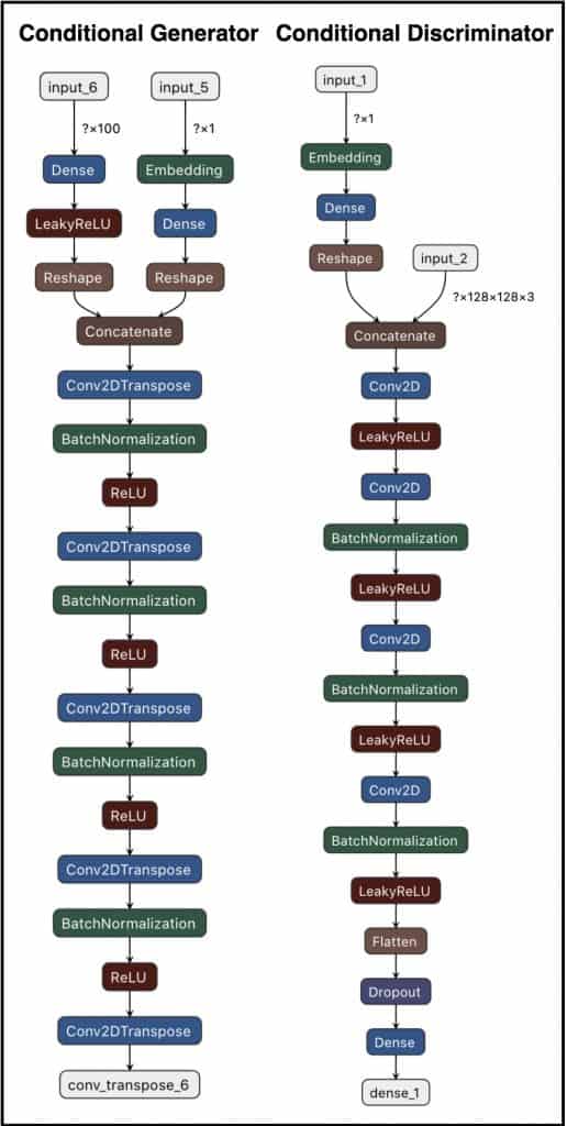
The idea is straightforward. Both generator and discriminator are fed a class label and conditioned on it, as shown in the above figures. All other components are exactly what you see in a typical  Generative Adversarial Networks framework, this being more of an architectural modification.

During the training of the CGAN: 

• The Generator is parameterized to learn and produce realistic samples for each label in the training dataset.
• The Discriminator learns to distinguish fake and real samples, given the label information. 
• However, their roles don’t change. The Generator and Discriminator continue to generate and classify images just like before, but with conditional auxiliary information.

Purpose of Conditional Generator and Discriminator

Generator

Ordinarily, the generator needs a noise vector to generate a sample. In a conditional generation, however, it also needs auxiliary information that tells the generator which class sample to produce.

Let’s call the conditioning label . The Generator uses the noise vector  and the label  to synthesize a fake example (, ) = | ( conditioned on , where is the generated fake example). This fake example aims to fool the discriminator by looking as similar as possible to a real example for the given label.

Now, it is not enough for the Generator to produce realistic-looking data; it is equally important that the generated examples also match the label. So, if a particular class label is passed to the Generator, it should produce a handwritten image . You can thus clearly see that the Conditional Generator now shoulders a lot more responsibility than the vanilla GAN or DCGAN.

Once the Generator is fully trained, you can specify what example you want the Conditional Generator to now produce by simply passing it the desired label. Want to see that in action? Feel free to jump to that section.

Discriminator

The Discriminator is fed both real and fake examples with labels. It learns to not just recognize real data from fake, but also zeroes onto matching pairs. A pair is matching when the image has a correct label assigned to it. The Discriminator finally outputs a probability indicating the input is real or fake. Its goal is to learn to:

• Accept all real sample label pairs.
• Reject all fake sample label pairs (the sample matches the label ).
• Also, reject all fake samples if the corresponding labels do not match.

For example, the Discriminator should learn to reject:

• The pair in which the generated image is , but the label was , regardless of the example being real or fake. The reason being it does not match the given label.
• All image-label pairs in which the image is fake, even if the label matches the image.

Enough of theory, right? Let’s apply it now to implement our own CGAN model. We would be training CGAN particularly on two datasets: The Rock Paper Scissors Dataset and the Fashion-MNIST Dataset. And implementing it both in TensorFlow and PyTorch.

Coding a Conditional GAN in TensorFlow

Dataset

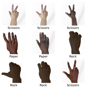
Use the Rock Paper Scissors Dataset. It consists of:

• Total 2,892 images of diverse hands in Rock, Paper and Scissors poses (as shown on the right).
• Each image is of size 300 x 300 pixels, in 24-bit color, i.e., an RGB image.
• These particular images depict hands from different races, age and gender, all posed against a white background.
• The hands in this dataset are not real though, but were generated with the help of Computer Generated Imagery (CGI) techniques.
• The dataset is part of the TensorFlow Datasets repository.

Note: All the implementations were carried out on an 11GB Pascal 1080Ti GPU.

Importing the Packages

#import the required packages
import cv2
import tensorflow as tf
from tensorflow.keras import layers
from IPython import display
import matplotlib.pyplot as plt
import numpy as np
import tensorflow_datasets as tfds
%matplotlib inline

Begin by importing necessary packages like TensorFlow, TensorFlow layers, matplotlib for plotting, and TensorFlow Datasets for importing the Rock Paper Scissor Dataset off-the-shelf (Lines 2-9).

Data Loading and Preprocessing

ds = tfds.load('RockPaperScissors', split='train', as_supervised=True, shuffle_files=True)

ds = ds.shuffle(1000).batch(128)

@tf.function
def normalization(tensor):
    tensor = tf.image.resize(
    tensor, (128,128))
    tensor = tf.subtract(tf.divide(tensor, 127.5), 1)
    return tensor

Click here to download the source code to this post

Loading the dataset is fairly simple; you can use the TensorFlow dataset module, which has a collection of ready-to-use datasets (find more information on them here). 

• Call the load function of TensorFlow dataset and pass the dataset name i.e., RockPaperScissors.
• The as_supervised=True flag ensures the returned dataset has a 2-tuple structure (input, label).
• Now that we have the dataset, in Line 12, shuffle the data and create batches of size 128, where we will train our model.
• Then in Lines 14-19, define a custom normalization function, which will be used during training. The function is quite simple: It resizes the original images of 300×300 dimension to 128×128 dimension and normalizes images from [0, 255] to [-1, 1].

Conditional Generator and Discriminator Architecture

Conditional Generator Implementation

# label input
con_label = layers.Input(shape=(1,))

# latent vector input
latent_vector = layers.Input(shape=(100,))

Thereafter, we define the TensorFlow input layers for our model. In the CGAN, because we not only feed the latent-vector but also the label to the generator, we need to specifically define two input layers:

• con_label – This is simply a (1,) vector, which expects one of three class labels as an input. 
• latent_vector –  This is the usual noise vector input that we have in other GAN networks. In this case, it is a (100,) vector.

def label_conditioned_generator(n_classes=3, embedding_dim=100):
    # embedding for categorical input
    label_embedding = layers.Embedding(n_classes, embedding_dim)(con_label)
    #print(label_embedding)
    # linear multiplication
    nodes = 4 * 4 
    label_dense = layers.Dense(nodes)(label_embedding)
    # reshape to additional channel
    label_reshape_layer = layers.Reshape((4, 4, 1))(label_dense)
    return label_reshape_layer

def latent_input(latent_dim=100):
    # image generator input
    nodes = 512 * 4 * 4
    latent_dense = layers.Dense(nodes)(latent_vector)
    latent_dense = layers.ReLU()(latent_dense)
    latent_reshape = layers.Reshape((4, 4, 512))(latent_dense)
    return latent_reshape

Recall that the Generator of CGAN is fed a noise-vector conditioned by a particular class label. Now, we implement this in our model by concatenating the latent-vector and the class label. To concatenate both, you must ensure that both have the same spatial dimensions.

We define two functions:

1. The label_conditioned_generator – It has an embedding layer, which is fed a categorical input. In our case, it’s one of the three classes, an integer ( 0 to 2 ). The embedding layer inputs the element’s index in your selected embedding and returns the corresponding embedding. It is widely used in Natural Language Processing (NLP).

a) Here, it turns the class label into a dense vector of size embedding_dim (100).

b) The label-embedding output is mapped to a dense layer having 16 units, which is then reshaped to [4, 4, 1] at Line 33.

2. The latent_input function – It is fed a noise vector of size 100, which is usually connected to a dense layer having 4*4*512 units, followed by a ReLU activation function. The output is then reshaped to a feature map of size [4, 4, 512].

# define the final generator model
def define_generator():
    latent_vector_output = label_conditioned_generator()
    label_output = latent_input()
    # merge label_conditioned_generator and latent_input output
    merge = layers.Concatenate()([latent_vector_output, label_output])
    
    x = layers.Conv2DTranspose(64 * 8, kernel_size=4, strides= 2, padding='same', kernel_initializer=tf.keras.initializers.RandomNormal(
    mean=0.0, stddev=0.02), use_bias=False, name='conv_transpose_1')(merge)
    x = layers.BatchNormalization(momentum=0.1,  epsilon=0.8, center=1.0, scale=0.02, name='bn_1')(x)
    x = layers.ReLU(name='relu_1')(x)
    
    x = layers.Conv2DTranspose(64 * 4, kernel_size=4, strides= 2, padding='same', kernel_initializer=tf.keras.initializers.RandomNormal(
    mean=0.0, stddev=0.02), use_bias=False, name='conv_transpose_2')(x)
    x = layers.BatchNormalization(momentum=0.1,  epsilon=0.8, center=1.0, scale=0.02, name='bn_2')(x)
    x = layers.ReLU(name='relu_2')(x)
    
    x = layers.Conv2DTranspose(64 * 2, 4, 2, padding='same', kernel_initializer=tf.keras.initializers.RandomNormal(
    mean=0.0, stddev=0.02), use_bias=False, name='conv_transpose_3')(x)
    x = layers.BatchNormalization(momentum=0.1,  epsilon=0.8,  center=1.0, scale=0.02, name='bn_3')(x)
    x = layers.ReLU(name='relu_3')(x)
  

    x = layers.Conv2DTranspose(64 * 1, 4, 2, padding='same', kernel_initializer=tf.keras.initializers.RandomNormal(
    mean=0.0, stddev=0.02), use_bias=False, name='conv_transpose_4')(x)
    x = layers.BatchNormalization(momentum=0.1,  epsilon=0.8,  center=1.0, scale=0.02, name='bn_4')(x)
    x = layers.ReLU(name='relu_4')(x) 
    
    
    out_layer = layers.Conv2DTranspose(3, 4, 2,padding='same', kernel_initializer=tf.keras.initializers.RandomNormal(
    mean=0.0, stddev=0.02), use_bias=False, activation='tanh', name='conv_transpose_6')(x)
    
    
   # define model
    model = tf.keras.Model([con_label, latent_vector], out_layer)
    return model

Focus especially on Lines 45-48, this is where most of the magic happens in CGAN.

• We initially called the two functions defined above.
• Concatenate them using TensorFlow’s concatenation layer. This layer inputs a list of tensors with the same shape except for the concatenation axis and returns a single tensor. In this case, we concatenate the label-embedding output [4, 4, 1] and latent output [4, 4, 512] into a joint representation of size [4, 4, 513].
• After that, we have a regular decoder-like structure with five Conv2DTranspose blocks, which upsample the [4, 4, 513] feature map or representation to an image of size [128, 128, 3]. Each block next upsamples the feature map by a factor of two.
• In addition to the upsampling layer, it also has a batch-normalization layer, followed by an activation function.

As we go deeper into the network, the number of filters (channels) keeps reducing while the spatial dimension (height & width) keeps growing, which is pretty standard.

Conditional Discriminator Implementation

# label input
con_label = layers.Input(shape=(1,))

# input image
inp_img = layers.Input(shape=(128,128,3))

The input to the conditional discriminator is a real/fake image conditioned by the class label. Hence, like the generator, the discriminator too will have two input layers. Only instead of the latent vector, here we have an input layer for the image with shape [128, 128, 3].

def label_condition_disc(in_shape=(128,128,3), n_classes=3, embedding_dim=100):
    # label input
    con_label = layers.Input(shape=(1,))
    # embedding for categorical input
    label_embedding = layers.Embedding(n_classes, embedding_dim)(con_label)
    nodes = in_shape[0] * in_shape[1] * in_shape[2]
    # scale up to image dimensions with linear layer
    label_dense = layers.Dense(nodes)(label_embedding)
    # reshape to a tensor
    label_reshape_layer = layers.Reshape((in_shape[0], in_shape[1], 3))(li)
    # image input
    return label_reshape_layer


def image_disc(in_shape=(128,128,3)):
    inp_image = layers.Input(shape=in_shape)
    return inp_image

The function label_condition_disc inputs a label, which is then mapped to a fixed size dense vector, of size embedding_dim, by the embedding layer. The output of the embedding layer is then fed to the dense layer, which has a number of units equal to the shape of the image 128*128*3. Then, the output is reshaped as a 3D Tensor, by the reshape layer at Line 93.

The image_disc function simply returns the input image.

def define_discriminator():
    label_condition_output = label_condition_disc()
    inp_image_output = image_disc()
    # concat label as a channel
    merge = layers.Concatenate()([inp_image_output, label_condition_output])
    
    x = layers.Conv2D(64, kernel_size=4, strides= 2, padding='same', kernel_initializer=tf.keras.initializers.RandomNormal(
    mean=0.0, stddev=0.02), use_bias=False, name='conv_1')(merge)
    x = layers.LeakyReLU(0.2, name='leaky_relu_1')(x)
    
    x = layers.Conv2D(64 * 2, kernel_size=4, strides= 3, padding='same', kernel_initializer=tf.keras.initializers.RandomNormal(
    mean=0.0, stddev=0.02), use_bias=False, name='conv_2')(x)
    x = layers.BatchNormalization(momentum=0.1,  epsilon=0.8, center=1.0, scale=0.02, name='bn_1')(x)
    x = layers.LeakyReLU(0.2, name='leaky_relu_2')(x)
    
    x = layers.Conv2D(64 * 4, 4, 3, padding='same', kernel_initializer=tf.keras.initializers.RandomNormal(
    mean=0.0, stddev=0.02), use_bias=False, name='conv_3')(x)
    x = layers.BatchNormalization(momentum=0.1,  epsilon=0.8, center=1.0, scale=0.02, name='bn_2')(x)
    x = layers.LeakyReLU(0.2, name='leaky_relu_3')(x)
      
    x = layers.Conv2D(64 * 8, 4, 3,padding='same', kernel_initializer=tf.keras.initializers.RandomNormal(
    mean=0.0, stddev=0.02), use_bias=False, name='conv_5')(x)
    x = layers.BatchNormalization(momentum=0.1,  epsilon=0.8, center=1.0, scale=0.02, name='bn_4')(x)
    x = layers.LeakyReLU(0.2, name='leaky_relu_5')(x)
  
 
    flattened_out = layers.Flatten()(x)
    # dropout
    dropout = layers.Dropout(0.4)(flattened_out)
    # output
    dense_out = layers.Dense(1, activation='sigmoid')(dropout)
    # define model


    # define model
    model = tf.keras.Model([inp_image_output, con_label], dense_out)
    return model

In Line 105, we concatenate the image and label output to get a joint representation of size [128, 128, 6]. The concatenated output is fed to the typical classifier-like architecture that consists of various conv blocks followed by dense layers to eventually achieve an output of how likely the input image is real or fake.

• The intermediate layers have Leaky-Relu, with a slope of 0.2, as the activation function.
• In the output layer but Sigmoid is the activation function. It generally gets an output in the range [0, 1].

Batchnorm layers are used in [2, 4] blocks. The last convolution block output is first flattened into a dense vector, then fed into a dropout layer, with a drop probability of 0.4. The dropout layer’s output is next fed to a dense layer, with a single unit classifying the input.

Loss Function

binary_cross_entropy = tf.keras.losses.BinaryCrossentropy()

Similarly as DCGAN, the Binary Cross-Entropy loss too helps model the goals of the two networks.

Generator Loss

def generator_loss(label, fake_output):
    gen_loss = binary_cross_entropy(label, fake_output)
    #print(gen_loss)
    return gen_loss

The generator_loss is calculated with labels as real_target (1), as you really want the generator to fool the discriminator and produce images close to the real ones.

Discriminator Loss

def discriminator_loss(label, output):
    disc_loss = binary_cross_entropy(label, output)
    #print(total_loss)
    return disc_loss

The discriminator loss has:

• The real (original images) output-predictions label as 1.
• Fake output predictions label as 0.

The discriminator loss is called twice while training the same batch of images: once for real images, then for the fakes.

Training the Conditional GAN

# Notice the use of `tf.function`
# This annotation causes the function to be "compiled".
@tf.function
def train_step(images,target):
    # noise vector sampled from normal distribution
    noise = tf.random.normal([target.shape[0], latent_dim])
    # Train Discriminator with real labels
    with tf.GradientTape() as disc_tape1:
        generated_images = conditional_gen([noise,target], training=True)

        
        real_output = conditional_discriminator([images,target], training=True)
        real_targets = tf.ones_like(real_output)
        disc_loss1 = discriminator_loss(real_targets, real_output)
        
    # gradient calculation for discriminator for real labels    
    gradients_of_disc1 = disc_tape1.gradient(disc_loss1, conditional_discriminator.trainable_variables)
    
    # parameters optimization for discriminator for real labels   
    discriminator_optimizer.apply_gradients(zip(gradients_of_disc1,\
    conditional_discriminator.trainable_variables))
    
    # Train Discriminator with fake labels
    with tf.GradientTape() as disc_tape2:
        fake_output = conditional_discriminator([generated_images,target], training=True)
        fake_targets = tf.zeros_like(fake_output)
        disc_loss2 = discriminator_loss(fake_targets, fake_output)
    # gradient calculation for discriminator for fake labels 
    gradients_of_disc2 = disc_tape2.gradient(disc_loss2, conditional_discriminator.trainable_variables)
    
    
    # parameters optimization for discriminator for fake labels        
    discriminator_optimizer.apply_gradients(zip(gradients_of_disc2,\
    conditional_discriminator.trainable_variables))
    
    # Train Generator with real labels
    with tf.GradientTape() as gen_tape:
        generated_images = conditional_gen([noise,target], training=True)
        fake_output = conditional_discriminator([generated_images,target], training=True)
        real_targets = tf.ones_like(fake_output)
        gen_loss = generator_loss(real_targets, fake_output)

    # gradient calculation for generator for real labels     
    gradients_of_gen = gen_tape.gradient(gen_loss, conditional_gen.trainable_variables)
    
    # parameters optimization for generator for real labels
    generator_optimizer.apply_gradients(zip(gradients_of_gen,\
    conditional_gen.trainable_variables))    

The training function is almost similar to the DCGAN post, so we will only go over the changes. In Line 152, we sample a noise vector of size [Batch_Size, 100], which is then fed to a dense layer.

During forward pass, in both the models, conditional_gen and conditional_discriminator, we input a list of tensors. We feed the noise vector and label during the generator’s forward pass, while real/fake image and label are input during the discriminator’s forward propagation.

That’s all you truly need to modify the DCGAN training function, and there you have your Conditional GAN function all set to be trained.

def train(dataset, epochs):
  for epoch in range(epochs):
    start = time.time()
    for image_batch in dataset:
      img = tf.cast(image_batch, tf.float32)
      imgs = normalization(img)
      train_step(imgs,target)

    print ('Time for epoch {} is {} sec'.format(epoch + 1, time.time()-start))


train(ds, 200)

Finally, we train our CGAN model in Tensorflow.

• The above train function takes the dataset ds with raw images and labels and iterates over a batch.
• Before calling the GAN training function, it casts the images to float32, and calls the normalization function we defined earlier in the data-preprocessing step.
• Then the normalized images and the target (labels) are passed to the train_step function, which is called at every new batch.
• We also pass the Epochs (200), as the parameter to the train function.

Results of Conditional GAN with TensorFlow

Once we have trained our CGAN model, it’s time to observe the reconstruction quality. More importantly, we now have complete control over the image class we want our generator to produce. Isn’t that great?

def generate_images(model, test_input, n_classes=3):
  # Notice `training` is set to False.
  # This is so all layers run in inference mode (batchnorm).
    output = None
    for label in range(n_classes):
        labels = tf.ones(10) * label
        predictions = model([labels, test_input], training=False)
        if output is None:
            output = predictions
        else:
            output = np.concatenate((output,predictions))
     
    nrow = 3
    ncol = 10
    fig = plt.figure(figsize=(25,25))
    gs = gridspec.GridSpec(nrow, ncol, width_ratios=[1, 1, 1,1, 1,1, 1, 1, 1, 1],
         wspace=0.0, hspace=0.0, top=0.2, bottom=0.00, left=0.17, right=0.845) 

    label_dict[np.array(labels)[0]])
    k = 0
    for i in range(nrow):
        for j in range(ncol):
            pred = (output[k, :, :, :] + 1 ) * 127.5
            pred = np.array(pred)  
            ax= plt.subplot(gs[i,j])
            ax.imshow(pred.astype(np.uint8))
            ax.set_xticklabels([])
            ax.set_yticklabels([])
            ax.axis('off')
            k += 1   

    plt.show()

• The generate_images function takes the generator model, the noise vector and the class labels as input. 
• We iterate over each of the three classes and generate 10 images. As the model is in inference mode, the training argument is set False.
• The predictions are generally stored in a NumPy array, and after iterating over all three classes, the array’s output has a shape of [30, 128, 128, 3].
• Then to plot these images in a grid, where the images of the same class are plotted horizontally, we leverage the matplotlib module.

num_examples_to_generate = 10
latent_dim = 100
n_classes = 3
noise = tf.random.normal([num_examples_to_generate, latent_dim])

generate_images(conditional_gen, noise,  n_classes)

We generally sample a noise vector from a normal distribution, with size [10, 100]. Next, feed that into the generate_images function as a parameter, along with the generator model and the number of classes.

From the above images, you can see that our CGAN did a pretty good job, producing images that indeed look like a rock, paper, and scissors. Not to forget, we actually produced these images based on our preference for the particular class we wanted to generate; the generator did not produce them arbitrarily.

Coding a Conditional GAN in PyTorch

In this section, we will implement the Conditional Generative Adversarial Networks in the PyTorch framework, on the same Rock Paper Scissors Dataset that we used in our TensorFlow implementation.

Data Loading and Preprocessing

train_transform = transforms.Compose([
    transforms.Resize(128),
    transforms.ToTensor(),
    transforms.Normalize([0.5,0.5,0.5], [0.5,0.5,0.5])])
train_dataset = datasets.ImageFolder(root='rps', transform=train_transform)
train_loader = torch.utils.data.DataLoader(dataset=train_dataset, batch_size=batch_size, shuffle=True)

In PyTorch, the Rock Paper Scissors Dataset cannot be loaded off-the-shelf.

• Begin by downloading the particular dataset from the source website.
• Once downloaded, use the ImageFolder module to load the dataset.
• Apply a total of three transformations: Resizing the image to 128 dimensions, converting the images to Torch tensors, and normalizing the pixel values in the range [-1, 1].
• Finally, prepare the training dataloader by feeding the training dataset, batch_size, and shuffle as True. You will recall that to train the CGAN; we need not only images but also labels. Ensure that our training dataloader has both.

Conditional Generator Implementation

class Generator(nn.Module):
    def __init__(self):
        super(Generator, self).__init__()
        
     
        self.label_conditioned_generator = 
        nn.Sequential(nn.Embedding(n_classes, embedding_dim),
                      nn.Linear(embedding_dim, 16))
        
    
        self.latent = 
        nn.Sequential(nn.Linear(latent_dim, 4*4*512),
                                   nn.LeakyReLU(0.2, inplace=True))
           

        self.model = 
        nn.Sequential(nn.ConvTranspose2d(513, 64*8, 4, 2, 1, bias=False),
                      nn.BatchNorm2d(64*8, momentum=0.1,  eps=0.8),
                      nn.ReLU(True),
                      nn.ConvTranspose2d(64*8, 64*4, 4, 2, 1,bias=False),
                      nn.BatchNorm2d(64*4, momentum=0.1,  eps=0.8),
                      nn.ReLU(True), 
                      nn.ConvTranspose2d(64*4, 64*2, 4, 2, 1,bias=False),
                      nn.BatchNorm2d(64*2, momentum=0.1,  eps=0.8),
                      nn.ReLU(True), 
                      nn.ConvTranspose2d(64*2, 64*1, 4, 2, 1,bias=False),
                      nn.BatchNorm2d(64*1, momentum=0.1,  eps=0.8),
                      nn.ReLU(True), 
                      nn.ConvTranspose2d(64*1, 3, 4, 2, 1, bias=False),
                      nn.Tanh())

    def forward(self, inputs):
        noise_vector, label = inputs
        label_output = self.label_conditioned_generator(label)
        label_output = label_output.view(-1, 1, 4, 4)
        latent_output = self.latent(noise_vector)
        latent_output = latent_output.view(-1, 512,4,4)
        concat = torch.cat((latent_output, label_output), dim=1)
        image = self.model(concat)
        #print(image.size())
        return image

The implementation of a conditional generator consists of three models:

• The label_conditioned_generator first takes the class label as input, then feeds it to the embedding layer of 100 dimensions, followed by a dense or linear layer that has 16 neurons.
• The latent model generally has a dense layer with 4*4*512 neurons. These are fed noise or latent vector of 100 dimensions, followed by a LeakyRelu activation.
• The third model is then fed to a concatenated output ( [513, 4, 4] ) of the previous two models. It subsequently outputs an image of size [3, 128, 128].

Be it PyTorch or TensorFlow, the architecture of the Generator remains exactly the same: number of layers, filter size, number of filters, activation function etc.

The third model has in total 5 blocks, and each block upsamples the input twice, thereby increasing the feature map from 4×4, to an image of 128×128.

Conditional Discriminator Implementation

class Discriminator(nn.Module):
    def __init__(self):
        super(Discriminator, self).__init__()
        
    
        self.label_condition_disc = 
        nn.Sequential(nn.Embedding(n_classes, embedding_dim),
                      nn.Linear(embedding_dim, 3*128*128))
             
        self.model = 
        nn.Sequential(nn.Conv2d(6, 64, 4, 2, 1, bias=False),
                      nn.LeakyReLU(0.2, inplace=True),
                      nn.Conv2d(64, 64*2, 4, 3, 2, bias=False),
                      nn.BatchNorm2d(64*2, momentum=0.1,  eps=0.8),
                      nn.LeakyReLU(0.2, inplace=True),
                      nn.Conv2d(64*2, 64*4, 4, 3,2, bias=False),
                      nn.BatchNorm2d(64*4, momentum=0.1,  eps=0.8),
                      nn.LeakyReLU(0.2, inplace=True),
                      nn.Conv2d(64*4, 64*8, 4, 3, 2, bias=False),
                      nn.BatchNorm2d(64*8, momentum=0.1,  eps=0.8),
                      nn.LeakyReLU(0.2, inplace=True), 
                      nn.Flatten(),
                      nn.Dropout(0.4),
                      nn.Linear(4608, 1),
                      nn.Sigmoid()
                     )

    def forward(self, inputs):
        img, label = inputs
        label_output = self.label_condition_disc(label)
        label_output = label_output.view(-1, 3, 128, 128)
        concat = torch.cat((img, label_output), dim=1)
        #print(concat.size())
        output = self.model(concat)
        return output

Like the generator in CGAN, even the conditional discriminator has two models: one to feed the labels, and the other for images.

• The label_condition_disc model is fed one of the three labels, which is then mapped to embedding_dim=100. Followed by a linear layer, which next maps the 100-dimension output from the previous layer to a dimension of 3*128*128. But why should the linear layer have 3*128*128 neurons? That’s simple. We need to concatenate the label with the real or fake image, so the label feature has to match the image dimensions, i.e., 128*128 truly.
• The model is fed a concatenation of the input image and output of the previous model ([6, 128, 128]), after which it outputs a single value that tells you whether the input image is real or fake.

Training the Conditional GAN

Both the loss function and optimizer are identical to our previous GAN posts, so let’s jump directly to the training part of CGAN, which again is almost similar, with few additions. We will only discuss the extensions in training, so if you haven’t read our earlier post on GAN, consider reading it for a better understanding.

num_epochs = 200
for epoch in range(1, num_epochs+1): 

    D_loss_list, G_loss_list = [], []
   
    for index, (real_images, labels) in enumerate(train_loader):
        D_optimizer.zero_grad()
        real_images = real_images.to(device)
        labels = labels.to(device)
        labels = labels.unsqueeze(1).long()

      
        real_target = Variable(torch.ones(real_images.size(0), 1).to(device))
        fake_target = Variable(torch.zeros(real_images.size(0), 1).to(device))
      
        D_real_loss = discriminator_loss(discriminator((real_images, labels)), real_target)
        # print(discriminator(real_images))
        #D_real_loss.backward()
    
        noise_vector = torch.randn(real_images.size(0), latent_dim, device=device)  
        noise_vector = noise_vector.to(device)
        
       
        generated_image = generator((noise_vector, labels))
        output = discriminator((generated_image.detach(), labels))
        D_fake_loss = discriminator_loss(output,  fake_target)

    
        # train with fake
        #D_fake_loss.backward()
      
        D_total_loss = (D_real_loss + D_fake_loss) / 2
        D_loss_list.append(D_total_loss)
      
        D_total_loss.backward()
        D_optimizer.step()

        # Train generator with real labels
        G_optimizer.zero_grad()
        G_loss = generator_loss(discriminator((generated_image, labels)), real_target)
        G_loss_list.append(G_loss)

        G_loss.backward()
        G_optimizer.step()

As in the vanilla GAN, here too the GAN training is generally done in two parts: real images and fake images (produced by generator). However, there is one difference. Earlier, each batch sampled only the images from the dataloader, but now we have corresponding labels as well (Line 88). These will be fed both to the discriminator and the generator.

In Line 92, cast the datatype of labels to LongTensor for we are using an embedding layer in our network, which expects an index. So, it should be an integer and not float.

Note all the changes we do in Lines98, 106, 107 and 122; we pass an extra parameter to our model, i.e., the labels.

• In the generator, we pass the latent vector with the labels.
• In the discriminator, we feed the real/fake images with the labels.

In Line 114, we average the discriminator real and fake loss and then compute the gradients based on this average loss. You could also compute the gradients twice: one for real data and once for fake, same as we did in the DCGAN implementation.

Results of Conditional GAN with PyTorch

Now that you have trained the Conditional GAN model, let’s use its conditional generator to produce few images. Recall in the Variational Autoencoder post; you generated images by linearly interpolating in the latent space. Using the same analogy, let’s generate few images and see how close they are visually compared to the training dataset.

From the above images, you can see that our CGAN did a good job, producing images that do look like a rock, paper, and scissors.

Class-Conditional Latent-Space Interpolation in a Conditional GAN Trained on the Fashion-MNIST Dataset

Look at the image below. It shows the class conditional latent-space interpolation, over 10 classes of Fashion-MNIST Dataset.

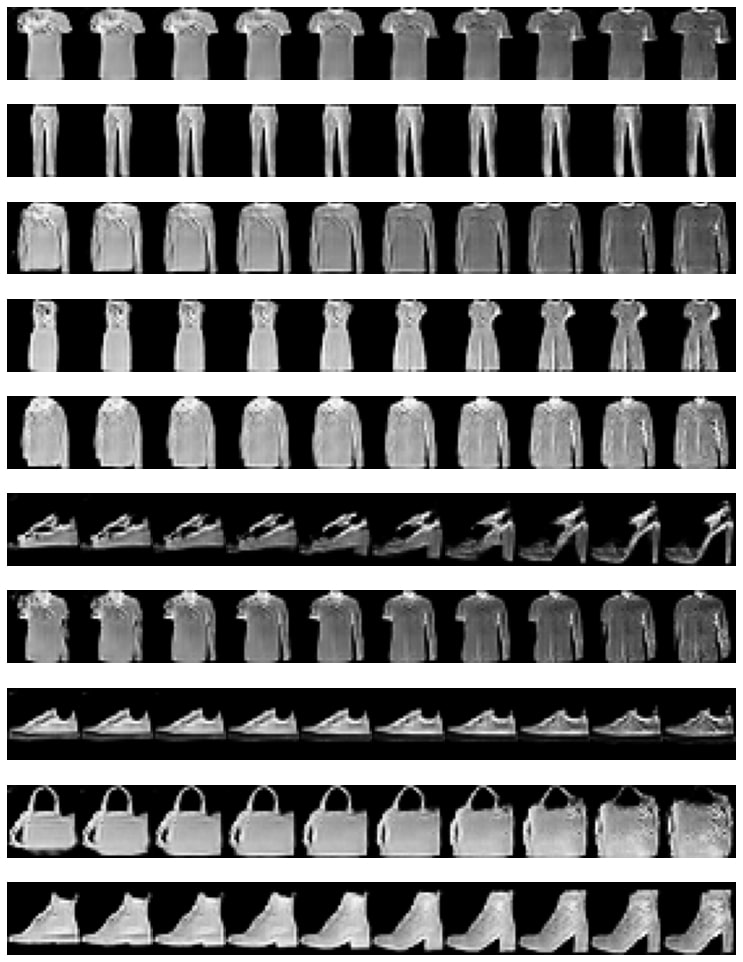
How to achieve this but?

• Firstly, train a CGAN on the Fashion-MNIST DataSet.
• Once trained, sample a latent or noise vector , of dimension [2, 100], and linearly interpolate around 10 vectors among them.
• Now feed these 10 vectors to the trained generator, which has already been conditioned on each of the 10 classes in the dataset.

That’s it. The images you finally get will look very similar to the real dataset.

In the above image, the latent-vector interpolation occurs along the horizontal axis. But to vary any of the 10 class labels, you need to move along the vertical axis.

Conclusion

Let’s quickly summarize:

1. You were first introduced to the Conditional GAN, a variant of  GAN that is trained by conditioning on a class label.
2. We then learned how a CGAN differs from the typical GAN framework, and what the conditional generator and discriminator tend to learn.
3. Afterwards we implemented a CGAN in TensorFlow, generating realistic Rock Paper Scissors and Fashion Images that were certainly controlled by the class label information.
4. To implement a CGAN, we then introduced you to a new Embedding layer that helped map the class labels to a fixed-size dense vector.
5. As a bonus, we also implemented the CGAN in the PyTorch framework.
6. We even showed how class conditional latent-space interpolation is done in a CGAN after training it on the Fashion-MNIST Dataset.

References

1. GANs in Action: Deep Learning with Generative Adversarial Networks by Jakub Langr and Vladimir Bok.