YOLO26 introduces a paradigm shift with native NMS-free inference. Discover how its One-to-One label assignment eliminates post-processing overhead for stable, real-time edge performance.
For years, the primary strategy for faster object detection has been to optimize the neural network architecture. Lighter convolutions, efficient attention mechanisms, and optimized feature pyramids helped reduce latency while maintaining accuracy. Yet even as models improved, a critical bottleneck remained at the very end of the pipeline: Non-Maximum Suppression (NMS).
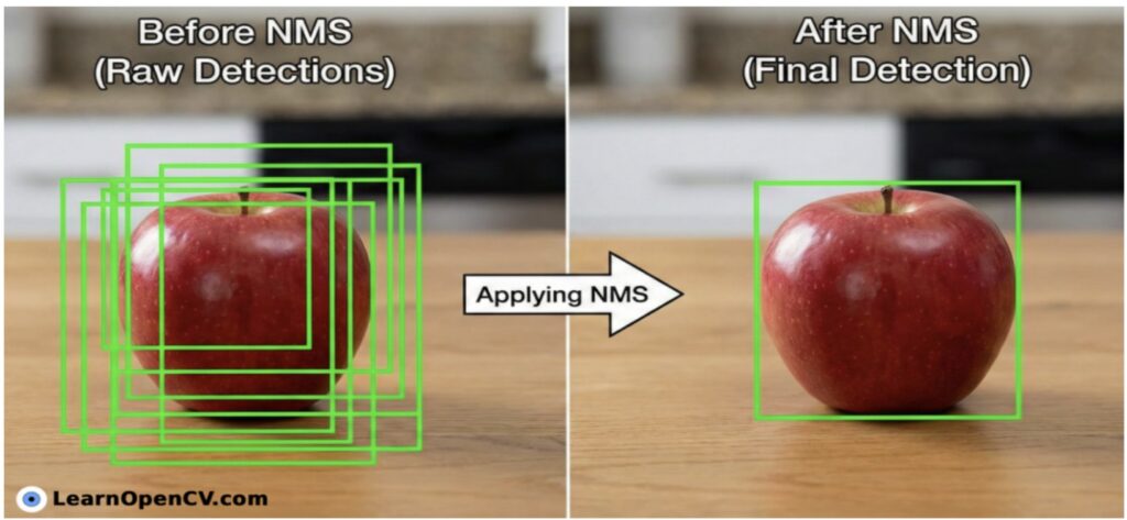
NMS is indispensable for removing duplicate detections, but it introduces practical complications. It depends on heuristic thresholds, behaves sequentially, and often executes outside the most optimized parts of the inference graph. On CPUs and edge accelerators, this step can dominate runtime and create data-dependent latency spikes.
YOLO26, released by Ultralytics on January 14, 2026, approaches the problem differently. Instead of cleaning predictions after they are made, the model is trained to produce a single, conflict-free box per object. This redesign enables true end-to-end inference and removes the need for NMS altogether.
What you’ll learn in this post:
- The Architecture: How YOLO26 achieves true end-to-end inference using a Dual-Head design.
- The Edge Optimization: Why removing Distribution Focal Loss (DFL) is critical for CPU performance.
- The Benchmarks: Analyzing the official performance metrics to understand the reported 43% CPU inference speedup.
Table of Contents
- Why NMS Becomes a Performance “Tax”
- Latency Variability
- How “One-to-One” Assignment Works
- What True End-to-End Export Looks Like
- Benchmarks & Conclusion
- Final Thoughts
- References
Filename: non-maximum-suppression-nms.jpg
Why NMS Becomes a Performance “Tax”
To appreciate the solution, the problem must first be understood. Why exactly is NMS such a hurdle for modern deployment?
The “One-to-Many” Legacy
Traditional detectors (like YOLOv5 through YOLOv8) are trained with a “One-to-Many” label assignment strategy. If the model detects a “Car,” it is encouraged to predict that car multiple times from slightly different anchor points. The benefit is that this maximizes recall (the probability of finding the object). The cost is that the raw output is not a clean list of objects, but a massive tensor containing thousands of redundant boxes (e.g., thousands of boxes for a standard 640×640 input).
The Serial Bottleneck
While GPUs excel at parallel processing, crunching those boxes simultaneously, NMS is fundamentally a sequential and sorting-heavy operation:
- Filter: Discard boxes below a confidence threshold.
- Sort: Rank the remaining boxes by score (an O(N log N) operation).
- Loop: Iterate through the sorted list, calculating Intersection over Union (IoU) and suppressing overlaps.
Although the Neural Network runs entirely on the GPU/NPU, the NMS step often falls back to the CPU. This creates a “ping-pong” effect where data moves between memory spaces, severely impacting throughput.
Latency Variability
A critical but often overlooked issue is that NMS runtime is data-dependent. If the camera sees a blank wall, NMS has almost nothing to sort. Inference is fast (e.g., 10ms). If the camera sees 50 pedestrians, NMS must sort and calculate IoU (Intersection Over Union) for hundreds of high-confidence boxes. Inference might spike to 25ms or more.
For robotics and safety-critical systems, this variable latency is unacceptable. Motion planning requires predictable timing. YOLO26 solves this by ensuring more deterministic latency, constant inference time, regardless of scene density.
Dive deeper into the logic behind NMS and IoU here – {https://learnopencv.com/non-maximum-suppression-theory-and-implementation-in-pytorch/ & https://www.youtube.com/watch?v=RgQbweTwrkU}
How “One-to-One” Assignment Works
If removing NMS offers such clear benefits, why was it not implemented sooner?
The historical challenge has been convergence. Forcing a model to predict only one box per object during training (One-to-One assignment) results in sparse supervision signals. The model struggles to learn because it is “punished” too often for slightly misaligned boxes, leading to poor accuracy.
The Evolution: From YOLOv10 to YOLO26
The architectural breakthrough required to solve this was first pioneered in YOLOv10 by Ao Wang et al. (Tsinghua University). Their research introduced the concept of Consistent Dual Assignments, a method to bridge the gap between rich training supervision and strict inference requirements. YOLO26 builds directly on this foundation, adopting the “One-to-One” philosophy while refining the implementation for greater stability and edge-device compatibility.
Dual-Head Training Mechanism
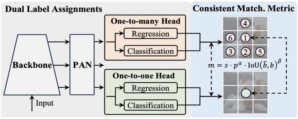
YOLO26 employs a Dual-Head Architecture during the training phase. Two separate heads share the same backbone and neck:
Head A: The “Teacher” (One-to-Many)
- Behavior: This acts as the traditional YOLO head, assigning multiple positive anchor points to a single ground-truth object.
- Purpose: It provides rich, dense gradients to the backbone, ensuring the model learns features quickly and robustly.
Head B: The “Student” (One-to-One)
- Behavior: This is the NMS-Free head. It uses a strict top-1 matching strategy, forcing the model to select the single best predicted box for each object.
- Purpose: It learns decisiveness, eliminating the need for post-processing.
The Consistent Matching Metric
The innovation lies in the alignment of these two heads. If they learn different representations, the model fails. YOLO26 uses a Consistent Matching Metric that forces the “One-to-One” head (the student) to align its predictions with the best candidates from the “One-to-Many” head (the teacher). Ideally, the shared backbone learns features that satisfy both the rich supervision of the Teacher and the strict requirements of the Student.
The Inference Switch
Once training is complete, Head A is discarded entirely. For deployment, only the backbone and the One-to-One Head are saved. Here is where YOLO26 diverges from its predecessor: While YOLOv10 used this architecture, it still relied on Distribution Focal Loss (DFL), which required complex mathematical decoding. YOLO26 replaces this with a Direct Regression Head. It removes the DFL entirely, meaning the model outputs raw coordinates directly without needing an expensive “Softmax” or integral calculation usually on the CPU (as visualized in Figure 3).
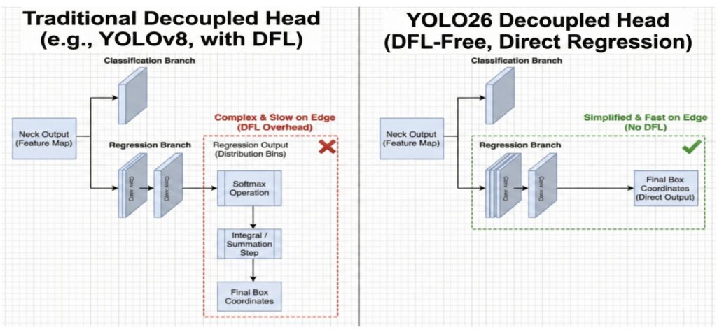
The Result: The neural network output is a clean, final set of boxes. No sorting, no IoU calculations, and no CPU fallback required.
What True End-to-End Export Looks Like
Architectural ideas are theoretical, but for deployment engineers, the computational graph tells the true story. Earlier YOLO pipelines typically required additional logic outside the network, such as custom NMS plugins in TensorRT or application-side filtering of dense prediction grids. Because YOLO26 removes both NMS and Distribution Focal Loss (DFL), the export process is radically simplified.
Step 1: Exporting the Model
The export script is typically simpler and does not require special arguments, such as nms=True, simplify=True, or custom post-processing flags. The network itself represents the full inference pipeline.
Installation
pip install ultralytics
Export
from ultralytics import YOLO

model = YOLO("yolo26n.pt")
path = model.export(format="onnx", opset=13)
Step 2: The Graph Comparison
To confirm that YOLO26 is truly end-to-end, you can inspect the ONNX graph. Visit Netron and upload your .onnx model file to explore the layers. { Link: https://netron.app }
- Traditional YOLO: The graph ends with multiple outputs, including box coordinates and class scores. Depending on the architecture, the model produces thousands of predictions per image. For instance, in anchor-based versions, a 40 × 40 grid with 3 anchors yields 4,800 predictions, whereas modern anchor-free models (like YOLOv11) produce up to ~8,400 predictions across all grids. These predictions must then be filtered using NMS.
- YOLO26: The graph ends with a single output tensor.
- Shape: [1, 300, 6] → batch size 1, 300 candidate boxes, 6 final values per box (4 coordinates, confidence and class_id).
- The model has already filtered duplicates, so only a confidence threshold is needed. No NMS is required.
Step 3: Running Inference
The Python inference loop no longer requires cv2.dnn.NMSBoxes. The data flows directly from the model to the application logic.
import onnxruntime
import numpy as np
import cv2
from google.colab.patches import cv2_imshow

# 1. Load image
# ===============================
image_path = "example.jpg"
original_img = cv2.imread(image_path)

if original_img is None:
    raise FileNotFoundError(f"Image not found at {image_path}")

h_orig, w_orig = original_img.shape[:2]

# 2. Preprocess
# ===============================
img = cv2.resize(original_img, (640, 640))
img = img.astype(np.float32) / 255.0
img = img.transpose(2, 0, 1)
image_data = np.expand_dims(img, 0)

# 3. Inference
# ===============================
session = onnxruntime.InferenceSession("yolo26n.onnx")
inputs = {session.get_inputs()[0].name: image_data}
outputs = session.run(None, inputs)[0]

# 4. Post-process & Draw
# ===============================
scale_x = w_orig / 640
scale_y = h_orig / 640
print("Inference successful! Detections:\n")

for box in outputs[0]:
    conf = float(box[4])
    if conf > 0.5:
        x1, y1, x2, y2 = box[:4]

        # rescale
        x1 = int(x1 * scale_x)
        y1 = int(y1 * scale_y)
        x2 = int(x2 * scale_x)
        y2 = int(y2 * scale_y)

        print(f"Box: {[x1,y1,x2,y2]}  Conf: {conf:.2f}")

        # draw
        cv2.rectangle(original_img, (x1, y1), (x2, y2), (0, 255, 0), 2)
        cv2.putText(original_img, f"{conf:.2f}", (x1, max(20, y1-10)),
                    cv2.FONT_HERSHEY_SIMPLEX, 0.6, (0,255,0), 2)

Figure 4: YOLO26 Inference Results. The model takes the raw image (left) and outputs precise detections (right). The lack of clutter confirms the effectiveness of the NMS-free design.
Filename: YOLO26-NMS-Free-Output.jpg
Benchmarks & Conclusion
YOLO26 is not merely a version increment; it is a specialized tool for edge computing. The removal of the “NMS Tax” and DFL math creates a specific performance profile.
Comparisons based on standard COCO validation on T4 GPU and CPU.
| Model | mAP (50-95) | Latency (GPU) | Latency (CPU) |
|---|---|---|---|
| YOLOv11n | 39.5 | 1.5 ± 0.0 ms | 56.1 ± 0.8 ms |
| YOLO26n | 40.9 | 1.7 ± 0.0 ms | 38.9 ± 0.7 ms |
The benchmark data reveals a clear optimization strategy. While GPU latency remains comparable, as the massive parallelization of high-end hardware absorbs the architectural changes, the CPU performance tells a different story. YOLO26n achieves a 40.9 mAP (surpassing YOLOv11n) while slashing CPU inference time from 56.1 ms down to 38.9 ms. This ~30-40% reduction in latency is transformative for edge deployment, proving that removing the NMS and DFL bottlenecks unlocks real-time performance on resource-constrained devices like Raspberry Pis and mobile phones, where every millisecond of compute directly impacts the user experience.
Final Thoughts
By standing on the shoulders of YOLOv10’s dual-assignment research and refining it with a DFL-free head, YOLO26 has finally broken the bottleneck. For the first time, the industry has a detector that is truly “What you train is what you get”. For engineers building on the edge, the era of tuning IoU thresholds is over. Object detection on resource-constrained hardware has entered a new phase—deterministic, streamlined, and ready for real-time applications.
References:
- YOLO26: Official Documentation {Link: Ultralytics YOLO26 – Ultralytics YOLO Docs}
- Google Collab Code Implementation { Link: https://colab.research.google.com/drive/19xvpMA- UxjmXTJ3TAsBUCZ2etgIk3FgX?usp=sharing }
- Related Article 1 {Link: https://arxiv.org/abs/2601.12882}
- Related Article 2 {Link: https://arxiv.org/abs/2509.25164}
- YOLOv10 Article {Link: https://arxiv.org/abs/2405.14458}

