


VGGT (Visual Geometry Grounded Transformer) leverages deep learning based representations to infer 3D structures from an image rather than traditional 2D based SfM pipelines. It provides a simplified, fast, reliable and versatile approach for 3D Reconstruction.
Traditional 3D Reconstruction methods heavily rely on visual geometry techniques such as SfM, MVS and iterative optimization using Bundle Adjustment (BA). However these methods are complex, time consuming and prone to errors. What if a model could bypass all these intermediary steps and directly can output a 3D scene, in less than a seconds?
Foundational models like DUSt3R and MASt3R by Naver Labs have pioneered this approach with a first of kind 3D foundational model, treating everything through a holistic 3D perspective. This radical idea, once thought impossible, has opened a whole possibilities of solvers in 3D tasks and had a significant impact especially on zero-shot 3D reconstruction with unconstrained (without known camera parameters) collection of images within few seconds.
But still these models need geometric post-processing techniques for multiple images fusing image pair reconstructions making them slow and computationally expensive. To address these challenges Meta unveiled a simple yet efficient VGGT pipeline generating reconstructions from a single image, a few or even up to hundreds of images in just single forward pass and thus eliminates geometric post processing entirely. VGGT outperforms DUSt3R and MASt3R by a huge margin.
If you’re someone just getting started with 3D computer vision, our series of articles will guide through the fundamentals of 3D Vision and Reconstruction.
- 3D Reconstruction with Gaussian Splatting and NeRF
- Stereo and Monocular Depth Estimation
- Understanding Camera calibration and Geometry.
- Visual SLAM
- DUSt3R: Dense 3D Reconstruction
- MASt3R and MASt3R-SfM
For a comprehensive overview about traditional Structure from Motion techniques and their limitations do check our DUSt3R and MASt3R article. In this article, we will cover VGGT paper explanation and interesting inference results.
- VGGT Model Architecture
- VGGT Training and Hyperparameters
- Code Walkthrough of VGGT Pipeline
- VGGT vs DUSt3R
- Limitations
- Key Takeaways
- Conclusion
- References
SfM (Structure from Motion): Traditional SfM tries to estimate the camera parameters and reconstruct sparse point clouds from collection of images of same scene. It involves multiple stages such as feature extraction, feature matching, triangulation and BA as implemented in tools like COLMAP.
MVS (Multi View Stereo): Dense Geometric Reconstruction generate dense point clouds with overlapping image pair but they require camera parameters to be known prior.
VGGT Model Architecture
VGGT is a feed forward neural network which directly predicts the 3D attributes without any post-processing optimization strategies. It is a large transformer (1.2B) with L = 24 layers that takes in a set of images  and predicts the output directly with a single transformer model.
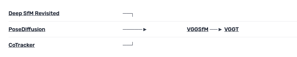
Meta VGGT is built on top of previous research works such as VGGSfM, CoTracker2 etc. aiming to collectively solve for all the tasks of these task-specific models thanks to its to its excellent 3D understanding and priors.
The overall VGGT transformer ( ) can be mathematically formulated as,

 – Camera parameters ;
 ![g = [q, t, f]](https://learnopencv.com/wp-content/ql-cache/quicklatex.com-bbc10ddc1721a14301a6cb0e32a280a5_l3.png)
assuming the image center is the camera’s principal point. – Depth Maps
 – Point Maps
 – Point Track Features of query points across 2D frames.
- Each input image is individually patched using DINO to extract a set of rich visual image embeddings
 . Additionally, a camera token is appended at beginning of each image tokens set to be aware of positional context.
 - These tokens are then aggregated across all the frames
 , and passed to the main transformer block which employs both global and frame-wise attention. The network utilizes Alternating Attention (AA) where the network alternates between focusing on tokens
  within individual frames and attending globally across all frames. This effectively balances local and global information resulting in significant improvements.
 - The authors reports that in the ETH3D Benchmarks, the AA approach outperforms both cross attention or only global self attention methods.
VGGT(
  (aggregator): Aggregator(
    (patch_embed): DinoVisionTransformer(
      (patch_embed): PatchEmbed(
        (proj): Conv2d(3, 1024, kernel_size=(14, 14), stride=(14, 14))
        (norm): Identity()
      )
      (blocks): ModuleList(
        (0-23): 24 x NestedTensorBlock(
 . . .
)
For frame-wise self-attention, each token attends only to tokens within same frame:

where M_{\text{frame} is a masking matrix that ensures each token can attend only to other tokens within same frame.
However in global attention, all tokens can attend to all other tokens across all the frames:

The DPT prediction head generates point maps, tracks and depthmaps while a separate camera head recovers camera intrinsics and extrinsics.
Similar to DUSt3R, the output pointmaps from VGGT are viewpoint invariant associateing each pixel with its corresponding 3D point in the scene. All views are aligned to a common coordinate system by choosing the first image’s camera pose as the reference frame. Pointmap representations enables seamless integrations with downstream applications particularly Gaussian Splatting.
VGGT solves for multiple 3D tasks such as:
1. Camera Parameter Estimation
 (camera_head): CameraHead(
    (trunk): Sequential(
      (0): Block( . . . )
          (token_norm): LayerNorm((2048,), eps=1e-05, elementwise_affine=True)
    (trunk_norm): LayerNorm((2048,), eps=1e-05, elementwise_affine=True)
    (embed_pose): Linear(in_features=9, out_features=2048, bias=True)
    (poseLN_modulation): Sequential(
      (0): SiLU()
      (1): Linear(in_features=2048, out_features=6144, bias=True)
    )
    (adaln_norm): LayerNorm((2048,), eps=1e-06, elementwise_affine=False)
    (pose_branch): Mlp(
      (fc1): Linear(in_features=2048, out_features=1024, bias=True)
      (act): GELU(approximate='none')
      (fc2): Linear(in_features=1024, out_features=9, bias=True)
      (drop): Dropout(p=0, inplace=False)
    )
  )
2. Dense Point Cloud Reconstruction
 (point_head): DPTHead(
    (norm): LayerNorm((2048,), eps=1e-05, elementwise_affine=True)
    (projects): ModuleList(
      (0): Conv2d(2048, 256, kernel_size=(1, 1), stride=(1, 1))
      (1): Conv2d(2048, 512, kernel_size=(1, 1), stride=(1, 1))
      (2-3): 2 x Conv2d(2048, 1024, kernel_size=(1, 1), stride=(1, 1))
    )
 . . .
         (output_conv1): Conv2d(256, 128, kernel_size=(3, 3), stride=(1, 1), padding=(1, 1))
      (output_conv2): Sequential(
        (0): Conv2d(128, 32, kernel_size=(3, 3), stride=(1, 1), padding=(1, 1))
        (1): ReLU(inplace=True)
        (2): Conv2d(32, 4, kernel_size=(1, 1), stride=(1, 1))
      )
    )
  )
3. Multi-View Depth Estimation
 (depth_head): DPTHead(
    (norm): LayerNorm((2048,), eps=1e-05, elementwise_affine=True)
    (projects): ModuleList(
      (0): Conv2d(2048, 256, kernel_size=(1, 1), stride=(1, 1))
      (1): Conv2d(2048, 512, kernel_size=(1, 1), stride=(1, 1))
      (2-3): 2 x Conv2d(2048, 1024, kernel_size=(1, 1), stride=(1, 1))
    )
. . .
      (output_conv1): Conv2d(256, 128, kernel_size=(3, 3), stride=(1, 1), padding=(1, 1))
      (output_conv2): Sequential(
        (0): Conv2d(128, 32, kernel_size=(3, 3), stride=(1, 1), padding=(1, 1))
        (1): ReLU(inplace=True)
        (2): Conv2d(32, 2, kernel_size=(1, 1), stride=(1, 1))
      ) ))
4. Point Tracking
(track_head): TrackHead(
    (feature_extractor): DPTHead(
      (norm): LayerNorm((2048,), eps=1e-05, elementwise_affine=True)
      (projects): ModuleList(
        (0): Conv2d(2048, 256, kernel_size=(1, 1), stride=(1, 1))
        (1): Conv2d(2048, 512, kernel_size=(1, 1), stride=(1, 1))
        (2-3): 2 x Conv2d(2048, 1024, kernel_size=(1, 1), stride=(1, 1))
      )
          )
 . . .
      (fmap_norm): LayerNorm((128,), eps=1e-05, elementwise_affine=True)
      (ffeat_norm): GroupNorm(1, 128, eps=1e-05, affine=True)
      (ffeat_updater): Sequential(
        (0): Linear(in_features=128, out_features=128, bias=True)
        (1): GELU(approximate='none')
      )
      (vis_predictor): Sequential(
        (0): Linear(in_features=128, out_features=1, bias=True)
      )
      (conf_predictor): Sequential(
        (0): Linear(in_features=128, out_features=1, bias=True)
      ))))
Features generated by pretrained VGGT can serve as a backbone for various downstream tasks, such as novel view synthesis and point tracking.
Tracking Points: Given a set of video frames and a query point, the tracking head predicts a set of 2D points from all images that correspond to the same 3D point. This is done by establishing correspondences by correlating features between the query image and all the matching points across all the frames in the sequence. From ablation studies it is found that when VGGT features are combined with existing point trackers like CoTracker, state-of-the results is achieved.


VGGT Training and Hyperparameters
VGGT solves multiple 3D tasks therefore the overall objective is converged by jointly optimizing with a multi-task loss:

The camera, depth and point maps losses have similar ranges but the tracking loss has to be downweighed by  =0.05
=0.05
Camera Loss

Depth Loss

Point Map Loss

Tracking Loss

The following table quickly summarizes the hyperparameters used during VGGT training,
| Hyperparameters | Values |
| Number of Layers (L) | 24 (global & frame-wise attention) |
| Model Size | ~1.2 billion parameters |
| Optimizer | AdamW |
| Iterations | 160K |
| Learning Rate Scheduler | Cosine Decay |
| Peak Learning Rate | 0.0002 |
| Warmup iterations | 8K |
| Batch size | Randomly sampled 2-24 frames |
| Max Input Dimension | 518 |
| Aspect Ratio Range | 0.33 to 1.0 |
| Image Augmentations | Color Jittering, Gaussian Blur, Grayscale |
While DUSt3R and MASt3R show promising results, they still require a global optimization post-processing step for better reconstruction quality and precise camera pose estimation.
In contrast, VGGT performs all tasks with shared backbone giving it a significant stride over task specific methods. Learning features across inter-related 3D tasks enhances overall accuracy, allowing VGGT to achieve on-par or superior performance compared to DUSt3R and MASt3R.
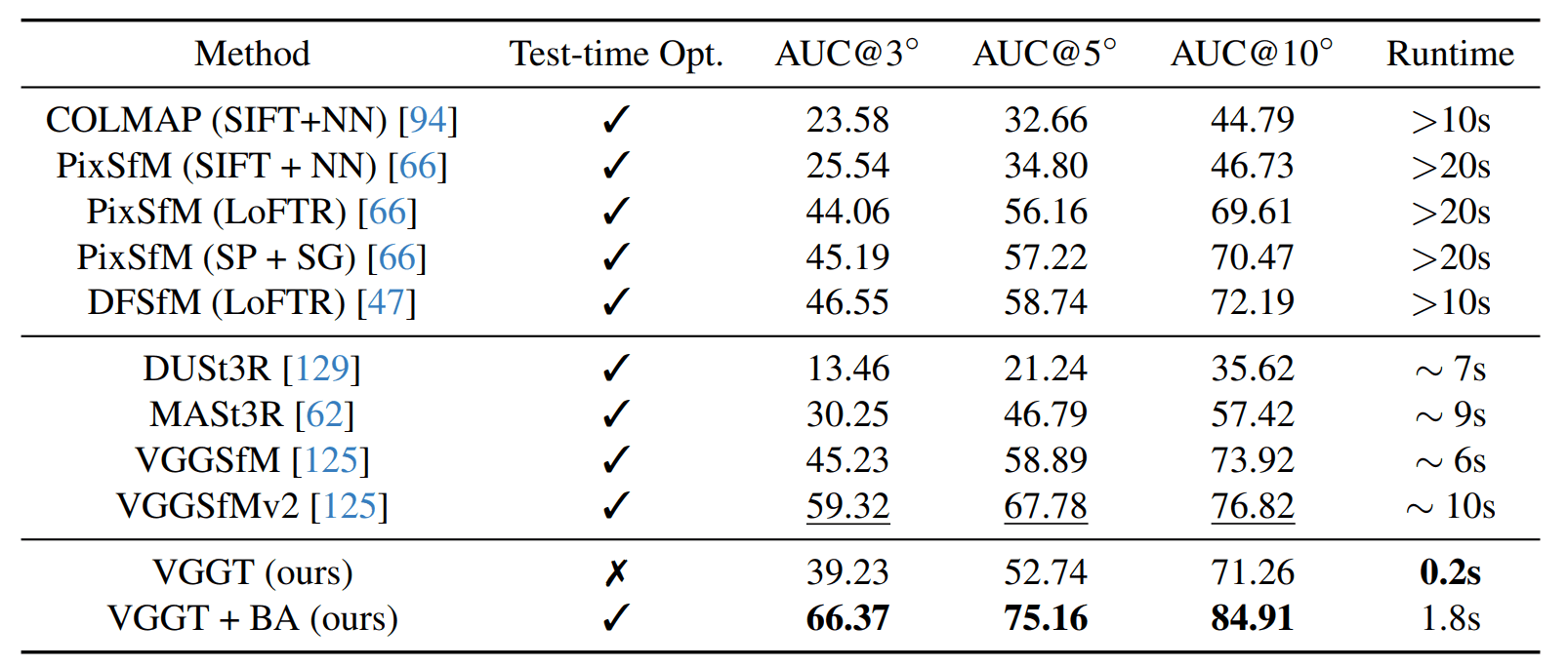
VGGT when combined with Bundle Adjustment, achieves superior performance to task-specific 3D models across multiple benchmarks.

Code Walkthrough of VGGT Pipeline
We tried inferencing on a 12GB VRAM GPU but as its a large model it didn’t fit in GPU. All the demos shown in the results are directly inferred using VGGT Hugging Face Spaces.
To run locally, clone the VGGT Repository and install dependencies
git clone git@github.com:facebookresearch/vggt.git
cd vggt
pip install -r requirements.txt
pip install -r requirements_demo.txt
To infer via gradio demo, simply run
python demo_gradio.py
python demo_viser.py --image_folder path/to/your/images/folder
Load Model
import torch
from vggt.models.vggt import VGGT
from vggt.utils.load_fn import load_and_preprocess_images

device = "cuda" if torch.cuda.is_available() else "cpu"
# bfloat16 is supported on Ampere GPUs (Compute Capability 8.0+)
dtype = torch.bfloat16 if torch.cuda.get_device_capability()[0] >= 8 else torch.float16

# Initialize the model and load the pretrained weights.
# This will automatically download the model weights the first time it's run, which may take a while.
model = VGGT.from_pretrained("facebook/VGGT-1B").to(device)

# (OR)
#model = VGGT()
#_URL = "https://huggingface.co/facebook/VGGT-1B/resolve/main/model.pt"
#model.load_state_dict(torch.hub.load_state_dict_from_url(_URL))
Preprocess the images by passing the image paths in a list
# Load and preprocess example images (replace with your own image paths)
image_names = ["path/to/imageA.png", "path/to/imageB.png", "path/to/imageC.png"]
images = load_and_preprocess_images(image_names).to(device)
We can directly perform forward pass by,
 # Predict attributes including cameras, depth maps, and point maps.
 predictions = model(images)
Or we can individually choose which attributes to predict via an aggregator network,
from vggt.utils.pose_enc import pose_encoding_to_extri_intri
from vggt.utils.geometry import unproject_depth_map_to_point_map

with torch.no_grad():
    with torch.cuda.amp.autocast(dtype=dtype):
        images = images[None]  # add batch dimension
        aggregated_tokens_list, ps_idx = model.aggregator(images)
        # len(aggregated_tokens_list) --> 24

    # Predict Cameras
    pose_enc = model.camera_head(aggregated_tokens_list)[-1]
    # pose_enc.shape --> (1, len(images), 9) --> (1, 3, 9)


    # Extrinsic and intrinsic matrices, following OpenCV convention (camera from world)
    extrinsic, intrinsic = pose_encoding_to_extri_intri(pose_enc, images.shape[-2:])
    # enstrinsic.shape --> (1, 3, 3, 4)
    # intrinsic.shape --> (1, 3, 3, 3)
    # Predict Depth Maps
    depth_map, depth_conf = model.depth_head(aggregated_tokens_list, images, ps_idx)
    # depth_map.shape --> (1, 3, 294, 518, 1)
    # depth_map.conf --> (1, 3, 394, 518)
We can generate the 3D Reconstruction directly from the point map of the network’s output,
    # Predict Point Maps
    point_map, point_conf = model.point_head(aggregated_tokens_list, images, ps_idx)
    # point_map.shape --> (1, 3, 294, 518, 1)
    # point_conf.conf --> (1, 3, 394, 518)
Alternatively, we can also recover the 3D correspondences with the camera parameters and depth map that we have obtained.
Interestingly, the authors quotes that “points maps derived from combining predicted depth map and camera poses is more accurate than directly using the output from dedicated pointmap head in VGGT” likely due to the more accurate camera parameters predicted by the camera head.
 # Construct 3D Points from Depth Maps and Cameras
 # which usually leads to more accurate 3D points than point map branch
 point_map_by_unprojection = unproject_depth_map_to_point_map(depth_map.squeeze(0),
                                                                extrinsic.squeeze(0),
                                                                intrinsic.squeeze(0))
Tracking with a query point
 # Predict Tracks
 # choose your own points to track, with shape (N, 2) for one scene
 query_points = torch.FloatTensor([[100.0, 200.0],
                                        [60.72, 259.94]]).to(device)
 track_list, vis_score, conf_score = model.track_head(aggregated_tokens_list, images, ps_idx, query_points=query_points[None])

# len(track_list) = 4
# vis_score.shape --> (1, 3, 2)
# conf_score.shape --> (1, 3, 2)
To visualize these tracklets,
from vggt.utils.visual_track import visualize_tracks_on_images
track = track_list[-1]
visualize_tracks_on_images(images, track, (conf_score>0.2) & (vis_score>0.2), out_dir="track_visuals")
Two green dots in the first and third frame are the common features that has been tracked for the given two query points.
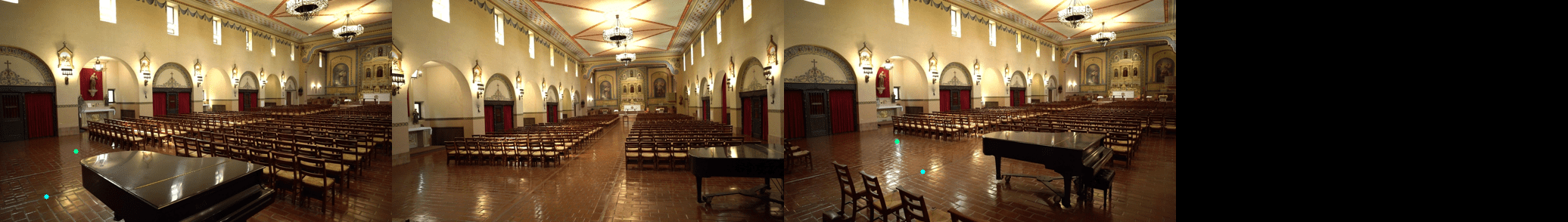
Single View
Two View
Multiple Views
VGGT vs DUSt3R
In terms of model architecture, the main difference between DUSt3R and VGGT is that VGGT has an additional tracking head and is capable of tracking query points across all frames.
In terms of speed and reconstruction quality VGGT performs better than DUSt3R.
| Views ( H100 GPU) | VGGT | DUSt3R |
| 1 (Single view) | <0.1 sec | <0.1 sec |
| 2 | <0.1 sec | <0.1 sec |
| 32 | <0.6 sec | >200 secs |
👉 Unlike DUSt3R which duplicates the image and process as a image pair for single view reconsruction, VGGT directly infers high-quality results from a single image.
In terms of model size, DUST3R can easily fit in a consumer grade GPUs occupying around 6GB for a single image ,whereas the default VGGT pipeline given required more than 12GB VRAM.
If we observe closely, we can see that the profile of cat structure is maintained intact in VGGT however in DUSt3R the cat appears boxy in shape.
Limitations
- While VGGT show strong generalization across 3D tasks, however it fails in scenarios where objects undergo flexible deformations or change shape over time, such as bending, stretching, or warping etc.
- Individuals and enterprises looking to integrate VGGT in your workflow and projects, should note that it is licensed under non-commercial (CC BY-NC-SA 4.0).
Key Takeaways
- VGGT is an single unified model where complex geometric algorithms or post processing techniques are replaced with feed forward networks grounding everything in 3D.
- VGGT ‘s simplicity and efficiency makes it idle for real-time applications compared to slow geometric-optimization based approaches.
- In few scenarios for larger scenes, we felt the fidelity and reconstruction quality of DUSt3R was better than VGGT in our experiments.
Conclusion
VGGT is a leap forward taking 3D Reconstruction to new heights. Following the success trails of DUSt3R and MASt3R which approach the problem with the perspective that everything is 3D in nature–using a single unified model for multiple downstream 3D tasks. VGTT takes this step further by enhancing the reconstruction quality and accuracy as well as being faster.
The future of 3D is promising and holds great potential, particularly in photo tourism and AR/VR. Imagine in an immersive experience where using devices like Vision Pro or Oculus, you can explore and navigate historical sites or monuments from your home as if you where physically there experiencing the same sense of presence as in reality.


100K+ Learners
Join Free OpenCV Bootcamp3 Hours of Learning