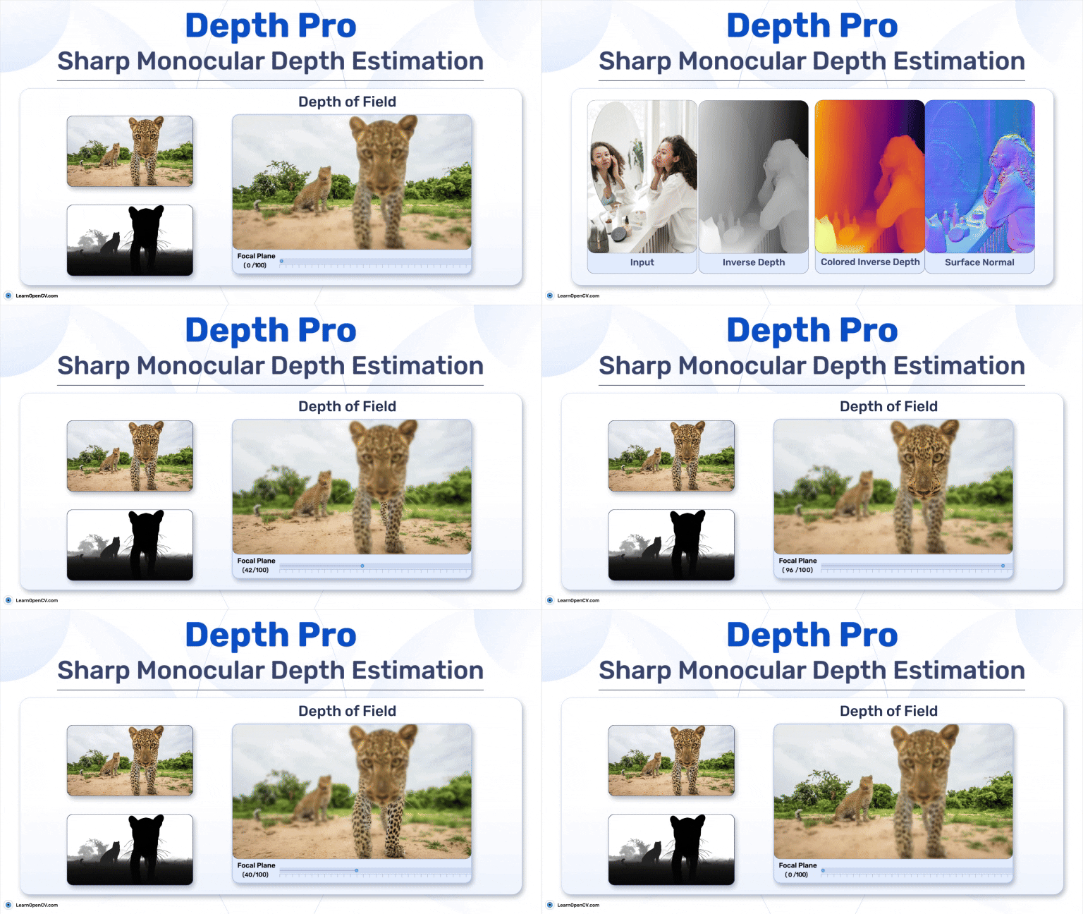
Depth Pro, is an foundational zero shot metric depth estimation model from Apple ML, nails at creating high resolution, sharp monocular metric depth maps in less than a second. Depth Pro achieves SOTA results in metric depth and outperfoms its competitors such as Depth Anything V2 and Marigold.
Imagine reviving those photos of a favorite childhood picnic, stored in your gallery. Well, why just imagine? With the image editing options in Google Photos, you can transform a still image and bring them to life with live-like motion edits of your choice and cherish those moments. The best part is, you don’t essentially need to have the camera metadata info of the original device with which they were shot. That’s the power of depth data inferred using modern monocular depth estimation.
The field of depth estimation has evolved significantly over the years. Think back to those good old days of Microsoft Kinetic on the Xbox, that brought an immersive and surreal gaming experience. Kinetic relied on the stereo-based cameras and had a pool of computer vision algorithms running behind the scenes to bring depth perception to life. While stereo cameras set the stage for depth applications, deep learning based monocular depth such as Depth Pro are simpler yet promising alternatives.
The topics discussed in this article are outlined as follows:
- Quick refresher to Monocular metric depth and its attributes
- Depth Pro Paper Explanation and Architectural details
- Inference with Depth Pro
- Comparing Depth Pro with models like DepthAnything and DepthCrafter
- Applications of Depth Data in Photo Editing
Individuals working at the intersection of computer vision and creative digital tools will find the application section to be highly engaging.
- A Primer to Monocular Depth Estimation
- Attributes of a Robust Monocular Depth Estimation Model
- Pointers from Depth Pro Paper
- DepthPro: Model Architecture
- Training strategy of Depth Pro By Apple ML
- Evaluation metrics and Benchmarks
- Code Walkthrough of Depth Pro Inference
- Depth Pro: Inference Results
- Estimating Metric Depth with Depth Pro
- Testing Depth Pro on Different Edge Cases
- Limitations of Depth Pro
- Comparison 1: Image Inference – Depth Pro v/s Depth Anything V2 v/s Marigold
- Comparison 2: Video Inference – Depth Pro v/s Depth Crafter
- Applications of Depth Map
- Key Takeaways
- Conclusion
If you’re just getting started with depth and stereo vision, we recommend you to check our series of articles on SpatialAI,
- Stereo Depth and Stereo Cameras
- Oak-D Stereo Camera
- Relative Depth estimation with DepthAnything
- Sapiens: Human Vision Models
A Primer to Monocular Depth Estimation
Typically, obtaining depth requires expensive LiDAR systems, or specialized stereo camera setup to capture multiple views of the same scene. However with SOTA monocular depth estimators, you can infer depth from a single image and can achieve on par results comparable to these hardware setups.
While there are classical heuristic approaches like Shape from X, that are still noteworthy, they rely on strong assumptions about the lighting or geometry about the scene, limiting their practicality for in-the-wild scenarios. That’s where deep learning based monocular depth estimation came into the play and shines in.
Monocular depth, though we deduce from a 2D image, it falls under representing a 3D info of the visual scene just like how humans perceive the world with cues and patterns. While there were earlier monocular depth models, the field started to pivot with Intel’s MiDAS and Depth Anything undergoing sophisticated advancements.
We knew that a semantic segmentation is a pixel-wise classification task, similarly a monocular depth estimation often is a pixel-wise regression task. It assigns values to each pixel of varying intensities helping to discern the object and the background either in absolute or relative scale.
1. Metric/Absolute Depth: Metric depth represents the depth in the real world for each pixel, where their intensity directly gauges the physical distance (in meters or centimeters) from the camera sensor to the object point corresponding to that pixel. eg: UniDepth, DepthPro
2. Relative Depth: Usually normalized between 0 to 1, indicates which pixels in the image are closer and which are farther away, to distinguish the foreground and background planes, without referring to real-world units of measurement. The results are sufficient for applications like image editing. eg: ZoeDepth , Depth Anything V2, Marigold
Attributes of a Robust Monocular Depth Estimation Model
- Generalization across diverse scenes: The model should perform consistently across various environments, whether it’s indoor or outdoor scenes. Training a single depth estimation model on all datasets typically deteriorates performance due to scaling differences between indoor and outdoor scenes especially in metric depth.
- Structural integrity and geometric features: The model should preserve the structural integrity and geometric features of the objects in the visual scene, leveraging cues like lighting, gradients, and textures.
- Independence from camera intrinsics: The model shouldn’t rely on camera specifics, which increases its usability in various applications.
- Sharp boundaries and artifact prevention: They should be able to handle occlusion boundaries and prevent artifacts like flying pixels and be able produce sharp boundaries.
- Fast and accurate: They should be computationally efficient, faster, and accurate.
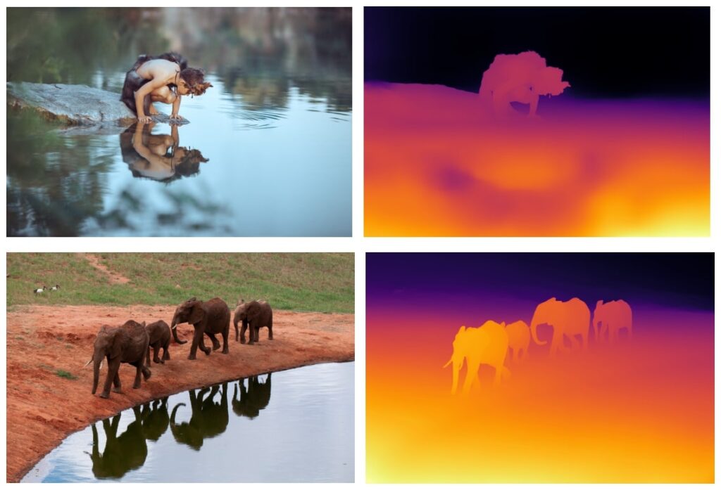
- Transparent and Reflective Surfaces: Typically, monocular depth estimation models struggle with transparent and reflective surfaces such as mirror, water and glass, as these exhibit complex lighting and refractive properties. The model should accurately understand the scene and deduce the inherent characteristics of the object, providing precise depth information and not falling short with mispredictions due to external reflections.
- Adaptability to varying focal lengths: Scenes captured with the same camera at varying focal lengths will have different perceptions of background distance. A good model should account for this variation and maintain consistent depth maps.
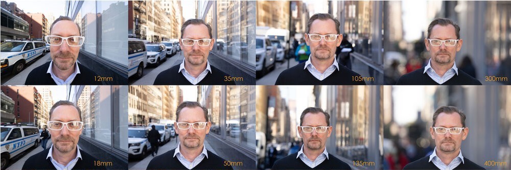
Source tonygale Sony Alpha Universe Community
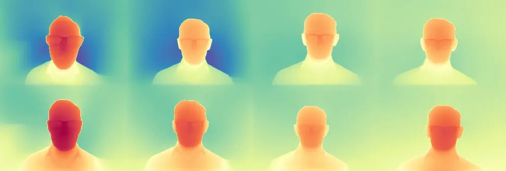
Pointers from Depth Pro Paper
Depth Pro is blazing fast and produces sharp high resolution depth maps. The paper reports that on a V100 GPU it takes just 0.3 sec to estimate the depth of an image. It natively produces a depth dim of 1536×1536 (~2.35 MP), with further upsampling to match the size of the input image.
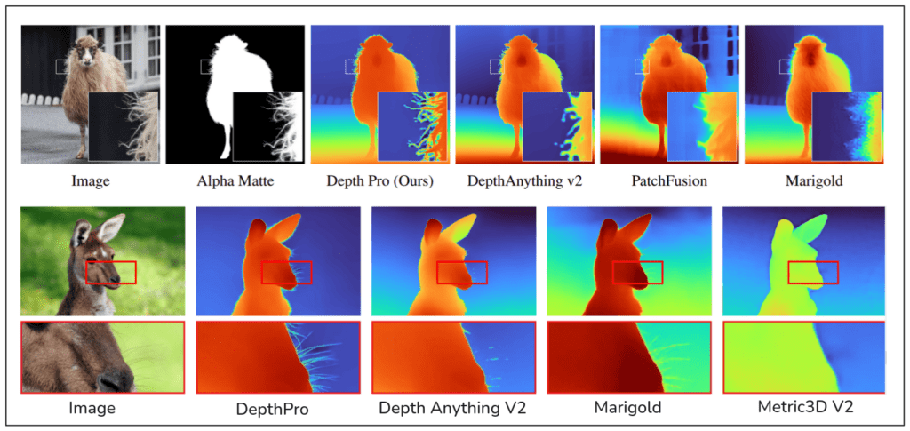
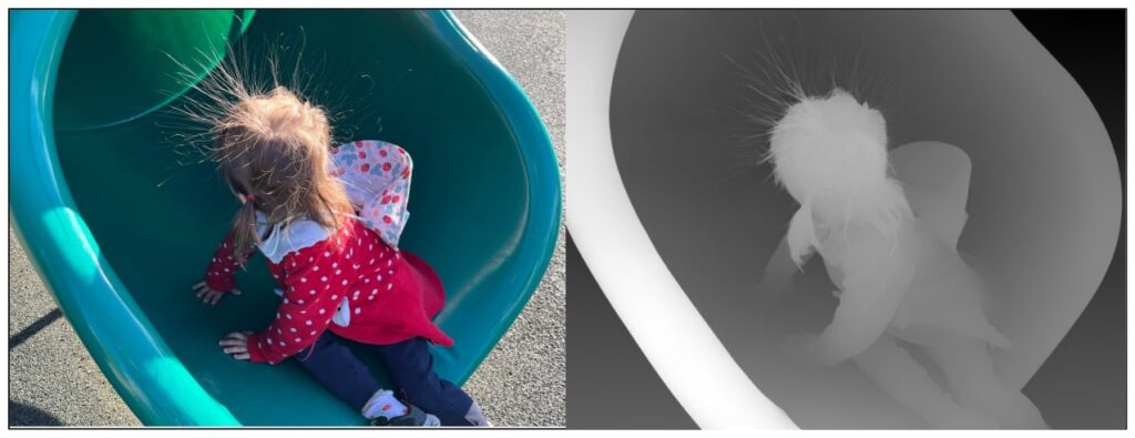
What makes Depth Pro stand out is its ability to produce high fidelity boundary delineation even for very thin structures like hair strands, or fur-like with high precision and recall. In contrast, Depth Anything V2 produces low fidelity and smoothened depth maps.
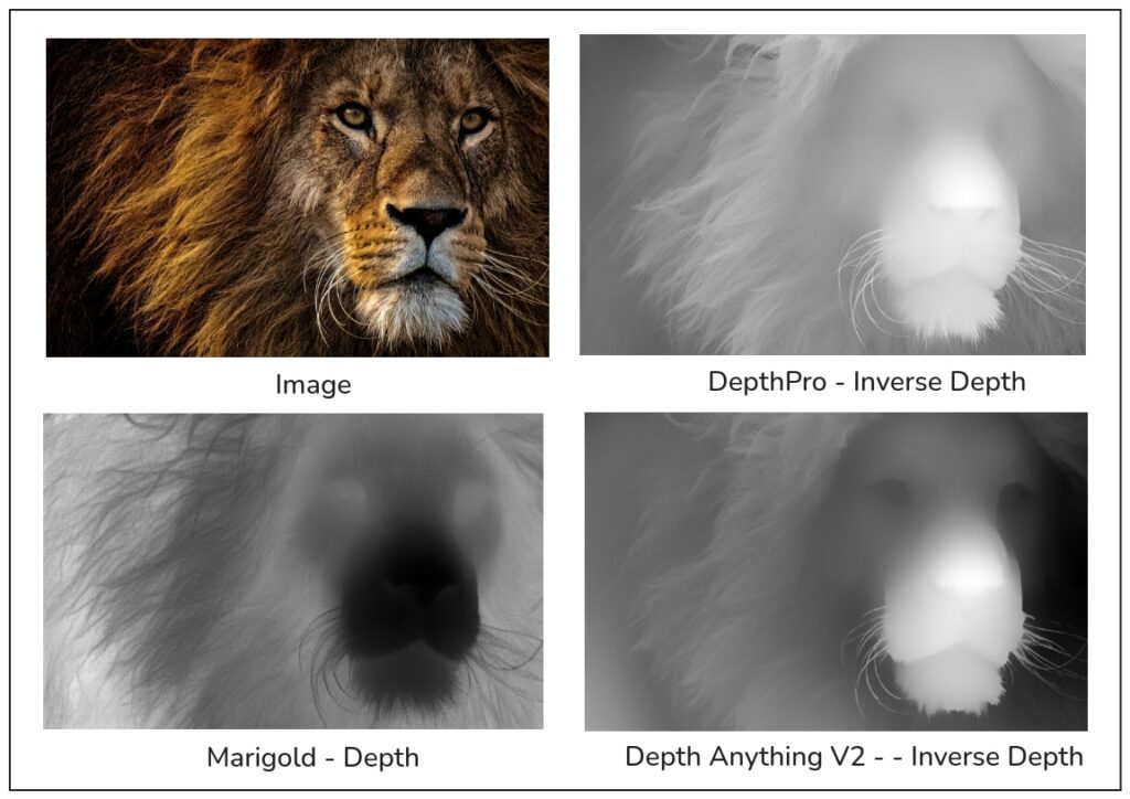
In the above example, we see that Marigold is also good in extracting the fur boundaries, though it yields finer-details than depth anything v2 it has noisy and grainy predictions which looks like a pencil sketch. Diffusion based depth models like Marigold have exceptional generalization as the rich latent space of theirs brings a lot of structural knowledge about the image, they remain slow due to multiple cycles or iterations of denoising. On the contrary, for sharp boundaries depth pro does not require any diffusion prior supervision or sophisticated multi-step task specific modules.
Unlike most monocular depth estimation models which are typically indomain and overfitted to a specific dataset constrained to either indoor or outdoor settings, Depth Pro consistently performs exceptionally well on in-the-wild images in dynamic environments making it the most preferred choice as a zero shot depth estimator.
The success of Depth Pro lies in its thoughtful design principles. It employs an efficient multi-scale vision transformer and incorporates a training protocol that combines real and synthetic datasets with sharp depth maps resulting in an unparalleled precision in boundary tracing.
The authors hint that depth pro design choices are specifically tailored for novel-view synthesis. In general, for novel view synthesis a good monocular depth estimation model should work zero shot and it should produce metric depth to reproduce shape and scenes. This allows it to determine the distances of objects within the scene without any requirement of camera intrinsics.
Depth Pro: Model Architecture
We knew that Transformers excels in capturing the global context due to their attention mechanism. However scaling Vision Transformers for high input resolution is computationally intensive due to their quadratic complexity O(n2).
As a workaround, instead of modifying any existing pretrained vision transformers and retraining the entire network, the authors approach cleverly to overcome this limitation by processing images at multiple scales (1536², 768² and 384²) and extracting their features using a naive ViT encoder at their disposal. Finally, these features from multiple scales are fused to obtain global context while still maintaining the low-level features.
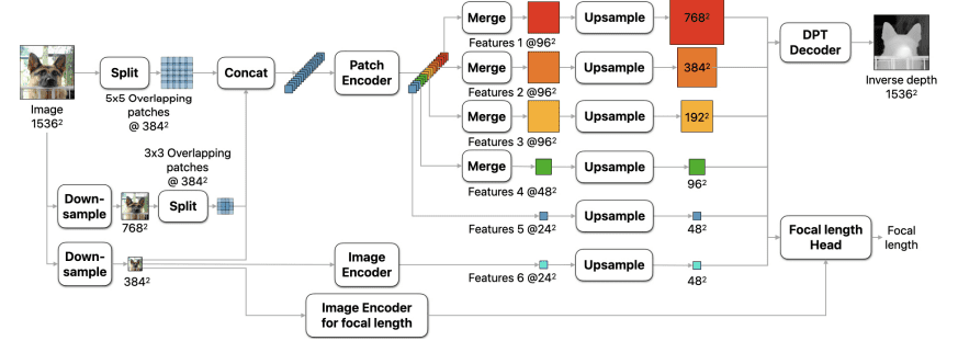
Multi Scale Vision Transformers
Depth Pro architecture primarily involves four main components:
- Image Encoder
- Patch Encoder
- DPT Decoder
- Focal length Head
Both the image encoders for depth and focal length are of ViT-L Dinov2 , the authors report that they performed exceptionally well compared to all other backbones from the timm library.
The patch encoder processes images as patches at different scales and fuses the learned representations across scales making them scale-invariant. These layers are shared to predict a single high-res dense map. Depth Pro operates at a fixed input resolution of 1536², and the output is upscaled to match the input image dimensions.
The input image is resized to 1536² and downsampled to 768² and 384². Note that these dimensions are multiples of 384. But why specifically 384? Because the authors leveraged a pretrained Dinov2 backbone from the timm library, which expects an input size of 384 allowing the use of backbone without any modifications.
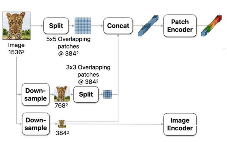
- High resolution: 1536 x 1536
- Mid resolution: 768 x 768
- Low resolution: 384 x 384
Then the high res and mid res image variants are split into overlapping patches to avoid seam with a patch size of 384².
For simplification lets consider dividing the high and mid res without overlap:
High Res: 1536²/384² = 4 x 4 patches,
Mid Res : 768² / 384² = 2 x 2 patches.
Now, if overlap is accounted for, we get:
- High Res: 5×5 overlapping patches @ 384²
- Mid Res: 3×3 overlapping patches @ 384²
- Low res: 1×1 patch @ 384²
Then the high, mid and low res images are concatenated and flattened into a 1D vector.
Patch Encoder
DepthPro(
  (encoder): DepthProEncoder(
    (patch_encoder): VisionTransformer(
      (patch_embed): PatchEmbed(
        (proj): Conv2d(3, 1024, kernel_size=(16, 16), stride=(16, 16))
This 1D input image vector is passed to a BeiT model with a patch size of 16×16 acts as a patch encoder. It encodes patches at three different scales and they are merged, producing an output feature map at five levels,
- Features 1@962 and Features2@962 are additional latent encodings hooked from the BeiT model’s high res patches with feature map size of 962 .
- Features 3@962 is of high res with feature map size of 962 (1536 x 1536 / 16 x 16)
- Features 4@482 is of mid res with feature map size of 482 (768 x 768 / 16 x 16)
- Features 5@242 is of low res with feature map size of 242 (384 x 384 / 16 x 16)
This multi-scale image representation helps Depth Pro to learn fine-grained features or local context in the given image.
(image_encoder): VisionTransformer(
(patch_embed): PatchEmbed(
   (proj): Conv2d(3, 1024, kernel_size=(16, 16), stride=(16, 16))
- Features 6@242 :
Additionally , low res version of the input image (3842) without any patch splitting is passed directly to the second image encoder acting like an anchor providing overall global context of the image.
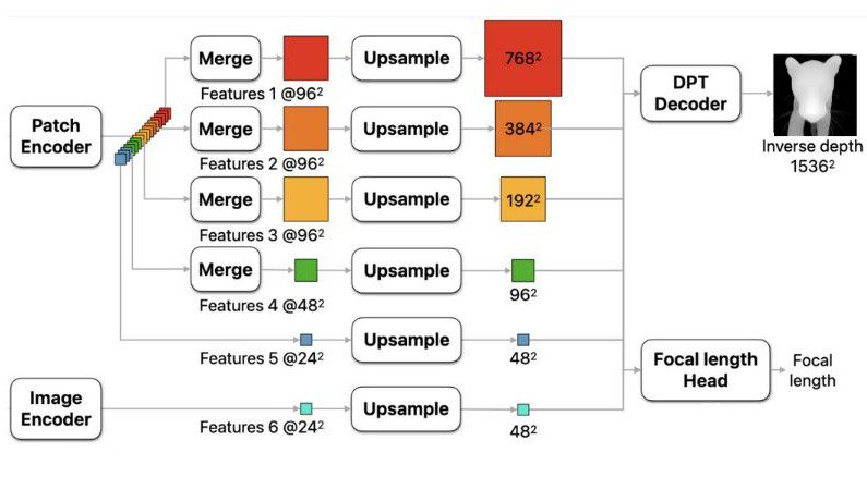
After encoding, these features are upsampled with specific scale factors to align their resolutions for final fusion via DPT Decoder with ConvTranspose2D:
- Feature 1: Scaled by a factor of 8
- Feature 2: Scaled by a factor of 4
- Features 3, 4, 5, 6: Scaled by a factor of 2
Used in most of the depth models like depth anything or MiDAS, DPT (Dense Prediction Transformer) is a decoder that leverages the Vision Transformer (ViT) for fine-grained pixel-wise depth prediction. Fusion blocks in DPT use residual convolutions to merge features and enhance resolution
(decoder): MultiresConvDecoder(
    (convs): ModuleList(. . .)
    (fusions): ModuleList(
      (0): FeatureFusionBlock2d(
		. . .)


(head): Sequential(
(0): Conv2d(256, 128, kernel_size=(3, 3), stride=(1, 1), padding=(1, 1))
(1): ConvTranspose2d(128, 128, kernel_size=(2, 2), stride=(2, 2))
(2): Conv2d(128, 32, kernel_size=(3, 3), stride=(1, 1), padding=(1, 1))
(3): ReLU(inplace=True)
(4): Conv2d(32, 1, kernel_size=(1, 1), stride=(1, 1))
(5): ReLU())
Depth Prediction Network
Depth Pro outputs an inverse depth map by default which is preferred for visualization purposes.
It represented as,
![]()
where C is Canonical inverse depth in metres(m).
Raw Depth: Closer pixel appear dark and farther pixels are appear white
Inverse Depth: Closer pixels appear white, farther pixels appear dark
![]()
Canonical Inverse Depth: Normalized or standardised inverse depth to make it consistent and interpretable as we fix scale based on:
- Min and max focal distance (absolute scale).
- Min and max intensity values (relative scale).
Dense metric depth: To compute dense metric depth, we need to scale the inverse depth with focal length (![]() for Horizontal FOV) and width(w) of the image.
for Horizontal FOV) and width(w) of the image.
This is formulated as:
![]()
where, ![]() is the dense metric depth,
is the dense metric depth, ![]() is the focal length predicted
is the focal length predicted
In most cases, the horizontal and vertical FOV of a camera will have the same focal length (f_px = f_py) as modern cameras use square pixels.
Focal Length Estimation Head
Focal length is the distance between the principal plane of the lens and the image plane (camera sensor) when the lens is focused on a subject at infinity. It is an important EXIF data of a camera that has to be known to scale depth which helps to determine how the 2D pixels will translate to a 3D distance of objects.
Usually monocular depth estimators do use the training dataset’s focal length to accurately project the 2D pixels into 3D point clouds. For instance, the Depth Anything V2 pipeline does use a focal length of 470.4 mm to convert its metric depth into point clouds.
Earlier zero shot metric depth models required camera intrinsics to be known to accurately produce depth maps. However, recent methods like UniDepth, introduces a network that has two separate modules for predicting depth and camera embedding, and the camera embedding is conditioned on depth map by concatenating the features to improve the depth quality which is independent of camera intrinsics about the training dataset.
Depth Pro, takes inspiration from Unidepth where focal length is obtained from the subnetwork of the model which estimates the focal length for an input image, this makes it possible to perform metric depth without the need for any source camera specific details. The FOVNetwork returns a single value for focal length in pixels.
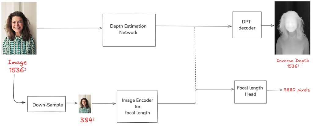
Why is the focal length a separate head?
In the Depth Pro pipeline, depth and focal length estimation are treated as separate tasks. If they were trained together, it would require balancing the two networks and optimizing them simultaneously. Therefore, using two networks enables a decoupled objective, allowing the depth and focal length networks to be trained independently on two completely different datasets without much reduction in performance metrics.
During inference, however, if a focal length for the input image is found in the EXIF data, it is preferred over the focal length estimated by the model’s FOV Head as its more reliable data than an estimated one, making it an obvious choice. The FOVNetwork does use a small convolutional head to predict the horizontal field of view.
(fov): FOVNetwork(
    (encoder): Sequential(
      (0): VisionTransformer(
		. . .
	)
(head): Sequential(
(0): Conv2d(128, 64, kernel_size=(3, 3), stride=(2, 2), padding=(1, 1))
(1): ReLU(inplace=True)
(2): Conv2d(64, 32, kernel_size=(3, 3), stride=(2, 2), padding=(1, 1))
(3): ReLU(inplace=True)
(4): Conv2d(32, 1, kernel_size=(6, 6), stride=(1, 1)))))
Training strategy of Depth Pro
Depth Pro is pretrained with a two stage training approach with a large mix of real and synthetic images to achieve high accuracy and sharp boundary delineation:
Stage 1: Training on Labelled Datasets
The model is initially trained on labeled datasets captured from lidar or stereo cameras that are available already over the internet. This makes the model to learn real world distributions for better generalization.
Stage 2: Fine-Tuning with Synthetic Datasets
To further improve the model for sharp outputs the model is further fine-tuned on synthetic datasets which have accurate sharp depth maps created using VFX or engines. A set of carefully chosen loss functions is used in conjunction with Scale and Shift Invariant (SSI) Loss with the objective to minimize the MAE loss. It improves precision in boundary regions and robust to scale and shifts of in-the-wild images.
Note: SSI Loss helps to disregard the scale and shifts variability with each sample in the training set. A loss function is taken into consideration that is independent of the scale and shifts of the data. This is done by transforming the depth value of the sample into disparity space and normalizing them between 0 and 1.
Evaluation metrics and Benchmarks of Apple Depth Pro
Depth Pro is a 504M parameter model which makes it to easily fit on a laptop with 6GiB VRAM . In comparison to its counterparts like Metric3D, Marigold requires more VRAM and takes more time for the same high res output but delivers low fidelity. Depth Pro strikes a balance between speed and performance.
Depth Pro outperforms all existing monocular depth estimation models achieving best average accuracy in zero-shot metric depth accuracy and highest F1 score, boundary recall (R) in zero-shot boundary accuracy, significantly.
From Table 1, we can see that Depth Pro operates on a completely different level, with an average rank of 2.5 (lower is better), indicating its aggregated performance across all the datasets.

The paper also proposes a new evaluation metric for sharp boundaries specifically to assess sharp boundaries in depth maps as existing benchmarks do not take this into account. To prepare a benchmark dataset for sharp boundary evaluation, existing binary segmentation or matting techniques were applied to prepare the ground truth for sharp boundaries depth map. As it is less time consuming to manually inspect a problematic segmentation mask than annotating them from scratch. The pixels at the edges of the binary segmentation mask are treated as object boundaries, which also solves the blurry edge problem commonly observed in monocular depth estimators.
As discussed, in Zero-shot boundary accuracy , depth pro ace across all the datasets its threshold accuracy (δ1: higher is better) highlighted in green which indicates that for any task where boundary precision matters depth pro is your go to model choice.

Now its time for hands on with coding, let’s go through the inference pipeline of Depth Pro and test the model’s aforementioned claims and actual performance when stressed under various conditions.
Code Walkthrough of Depth Pro Inference
To start out with Depth Pro locally simply, clone the repository, and install the required dependencies.
!git clone https://github.com/apple/ml-depth-pro.git
cd ml-depth-pro

#setup
!pip install -e .
You will need to download the pretrained checkpoint using the following bash command which will place the model under `ml-depth-pro/checkpoints/depth-pro.pt` folder.
source get_pretrained_models.sh
Image Inference – Usage
To run Depth Pro via cli,
!depth-pro-run -i image.jpg -o output_dir
The input can be an image or a directory containing multiple images, the output_dir will store the resulting inverse depth maps.
The following set of code is mostly adapted from ml-depth-pro/cli/run.py with few add-on snippets to calculate surface normal estimation from the raw depth.
Import Dependencies
import logging
from pathlib import Path
import cv2
import numpy as np
import PIL.Image
import torch
from matplotlib import pyplot as plt
from tqdm import tqdm

from depth_pro import create_model_and_transforms, load_rgb
We will load the model in half-precision and move it to “cuda”.
def run(args):
   """Run Depth Pro on a sample image."""

   # Load model.
   model, transform = create_model_and_transforms(
       device=get_torch_device(),
       precision=torch.half,
   )
   model.eval()

   image_paths = [args.image_path]
The input image is loaded as a PIL image using load_rgb, which returns f_px if it is obtained from the image metadata.
for image_path in tqdm(image_paths):
       # Load image and focal length from exif info (if found.).
       try:Parallax Effect with After Effects
           LOGGER.info(f"Loading image {image_path} ...")
           image, _, f_px = load_rgb(image_path)
       except Exception as e:
           LOGGER.error(str(e))
           continue
The input image is resized to 1536×1536, and basic transforms like ToTensor and Normalize are applied. The estimated depth is then resized to the original image dimensions.
 # Run prediction. If `f_px` is provided, it is used to estimate the final metric depth,
       # otherwise the model estimates `f_px` to compute the depth metricness.
       prediction = model.infer(transform(image), f_px=f_px)
All the inferences were carried out on a RTX4050 GPU with 6GiB VRAM, an i5 16 GB RAM machine. Each inference took less than 15 seconds per image, occupying 5GB of VRAM with half precision.
Depth Pro: Inference Results
1.Raw Depth
From the DPT Decoder head, the raw depth is extracted and is clipped between [0.1m;250m].
# Extract the depth.
depth = prediction["depth"].detach().cpu().numpy().squeeze()
max_depth_vizu = min(depth.max(), 1 / 0.1)
min_depth_vizu = max(depth.min(), 1 / 250)
depth_clipped = np.clip(depth, min_depth_vizu, max_depth_vizu)

depth_normalized = (depth_clipped - min_depth_vizu) / (max_depth_vizu - min_depth_vizu)

grayscale_depth = (depth_normalized * 255).astype(np.uint8)
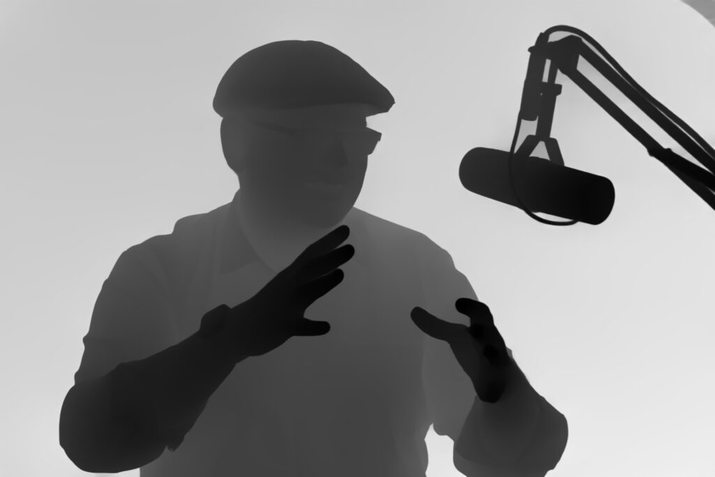
2. Inverse Depth
For better visualization, we can take an inverse of the raw depth which appears much more intuitive as we are mostly concerned about the foreground subjects rather than background. The inverse depth pixel values are normalized between [0.1m;250m] and scaled back to usual 8-bit grayscale format.
inverse_depth = 1 / depth
# Visualize inverse depth instead of depth, clipped to [0.1m;250m] range for better visualization.
max_invdepth_vizu = inverse_depth.max()
min_invdepth_vizu = inverse_depth.min()

inverse_depth_normalized = (inverse_depth - min_invdepth_vizu) / (
max_invdepth_vizu - min_invdepth_vizu
       )
inverse_depth_grayscale = (inverse_depth_normalized * 255).astype(np.uint8)
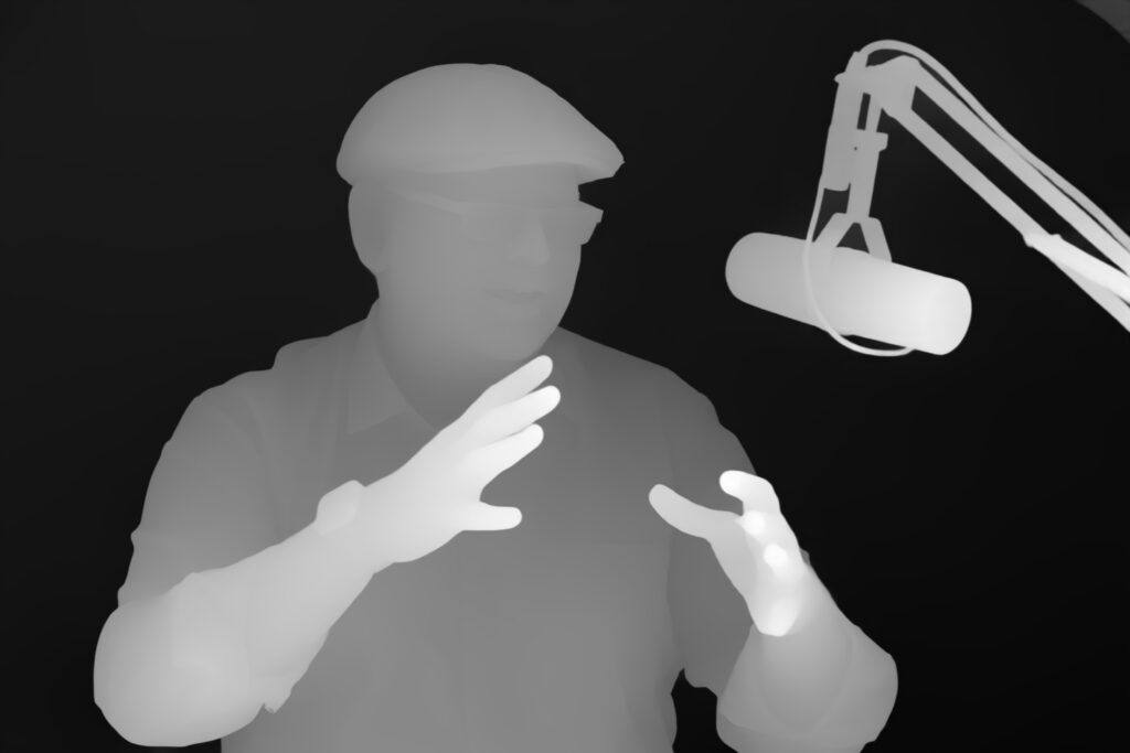
3. Color Inverse Depth
The inverse depth grayscale single channel depth map can be color-mapped with a cmap of “inferno” or other common options such as “viridis”, “turbo”.
# Save as color-mapped "turbo" jpg image.
cmap = plt.get_cmap("inferno")
color_depth = (cmap(inverse_depth_normalized)[..., :3] * 255).astype(
               np.uint8
           )
PIL.Image.fromarray(color_depth).save(
               inverse_cmap_output_file, format="JPEG", quality=90
           )

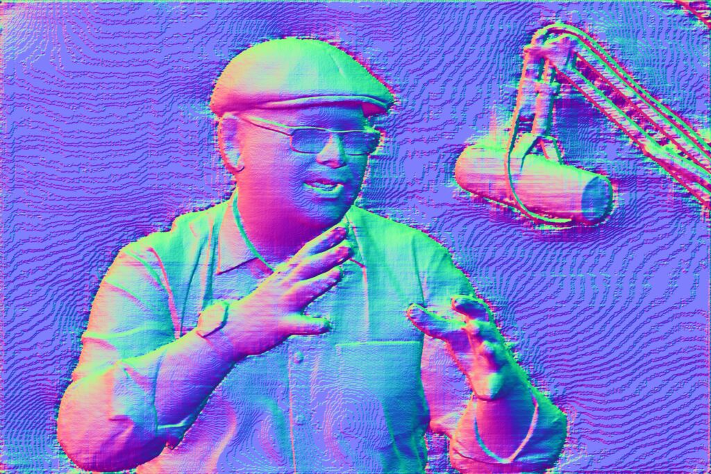
4. Surface Normal
Surface normal refers to the orientation of a subject in 3D space, where from camera ego blue represents the normals pointing towards the camera, green indicates right-facing normals and pink shades represents left normals. It provides local geometric cues that’s not immediately apparent in a depth map or segmentation mask.
Interestingly, surface normals can be estimated from raw depth by calculating the horizontal and vertical gradient using the Sobel operator with a kernel size like 7×7 here. An 8-bit RGB image is created by normalizing and scaling these normals for visualization.
#***************** SURFACE NORMAL ***********************
kernel_size = 7
grad_x = cv2.Sobel(depth.astype(np.float32), cv2.CV_32F, 1, 0, ksize = kernel_size)
grad_y = cv2.Sobel(depth.astype(np.float32), cv2.CV_32F, 0, 1, ksize = kernel_size)
z = np.full(grad_x.shape, 1)
normals = np.dstack((-grad_x, -grad_y, z))

normals_mag = np.linalg.norm(normals, axis= 2, keepdims=True)
with np.errstate(divide="ignore", invalid="ignore"):
      normals_normalized   = normals / (normals_mag + 1e-5)

normals_normalized = np.nan_to_num(normals_normalized, nan = -1, posinf=-1, neginf=-1)
normal_from_depth = ((normals_normalized + 1) / 2 * 255).astype(np.uint8)
5. Focal length in pixels
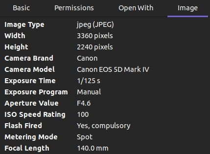
As discussed earlier, if we get the focal length in millimeters from the image EXIF data and convert it to focal length in pixels, it is chosen over the estimated f_px.
if f_px is not None:
           LOGGER.debug(f"Focal length (from exif): {f_px:0.2f}")
elif prediction["focallength_px"] is not None:
           focallength_px = prediction["focallength_px"].detach().cpu().item()
           print(f"Estimated focal length: {focallength_px}")
           LOGGER.info(f"Estimated focal length: {focallength_px}")
When the image focal length is converted to pixels, for 140mm we expect,
Focal length in pixels = (focal length in mm * image width in pixels) / sensor width in mm
The Canon EOS 5D Mark IV has a sensor width of 36mm,
Thus, ![]() = 140 x 3360 / 36 = 13066 pixels
= 140 x 3360 / 36 = 13066 pixels
Estimated focal length: ~9729.327 pixels returned by the Depth Pro FOVNetwork.
Absolute Difference = [Estimated Focal Length (pixels) – Calculated Focal Length (pixels)] = 13066 – 9729.33 = 3336.67 pixels
Percentage Difference = (Absolute Difference / Calculated Focal Length (pixels)) x 100% = (3336.67 / 13066) x 100% = 25.54%
Clearly there is a discrepancy between the actual focal length in pixels expected and the estimated focal length by Depth Pro FOV Head.
6. Sharp Depth Maps
Estimating Metric Depth with Depth Pro
Interactive OpenCV Window
For an interactive OpenCV Window demo scripts hit the “download code” button.
Let’s test the robustness of Depth Pro in estimating the physical distance of each point on an object from the camera.
Case 1: Actual Distance: 67 cm; Estimated Distance: ~ 68 to 71 cm
To do this, we placed a box at a distance of 67cm away from the table and captured it using a fixed mobile camera. The distance between the object and table is measured with metric tape for reference.

We observed that the model approximated the range around 68-71 cm when hovered over the cardboard box, which is impressive. However in some cases, we had failures possibly due to how the image is captured. One will need to do extensive testing for any real world use cases with depth pro for metric depth.
Case 2: Actual Distance: 100 cm ; Estimated Distance: ~110cm
The lowest plane / internal bottom of the box’s actual distance is 100cm , but DepthPro’s depth map estimates the points on that plane to be around 110cm.

Testing Depth Pro on Different Edge Cases
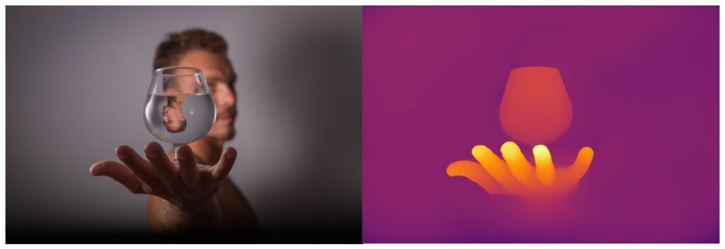
1.Glass Subjects

2. Inside Water

3. Water Reflections
Depth Pro performs exceptionally well in distinguishing water reflections from real subjects, by not mistaking reflections of the boy or the elephants in the water as an actual subjects.
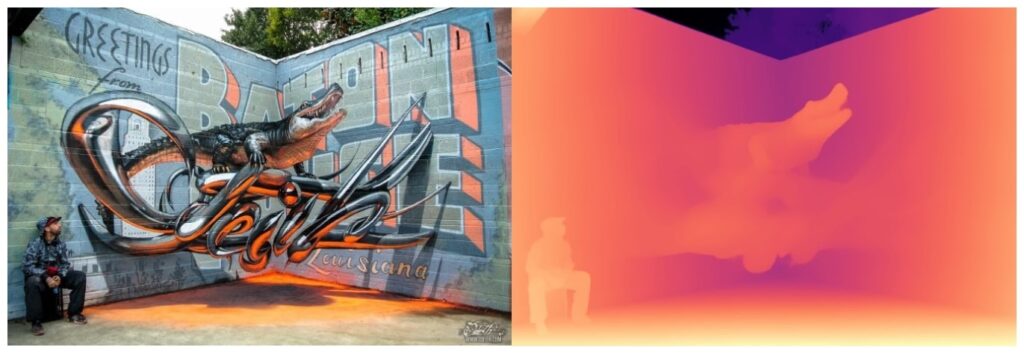
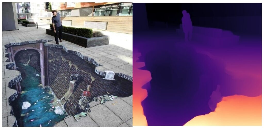
4. Illusion
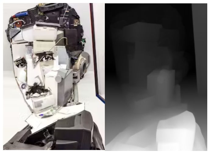
courtesy Patrik Proško
Limitations of Depth Pro
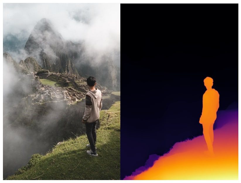
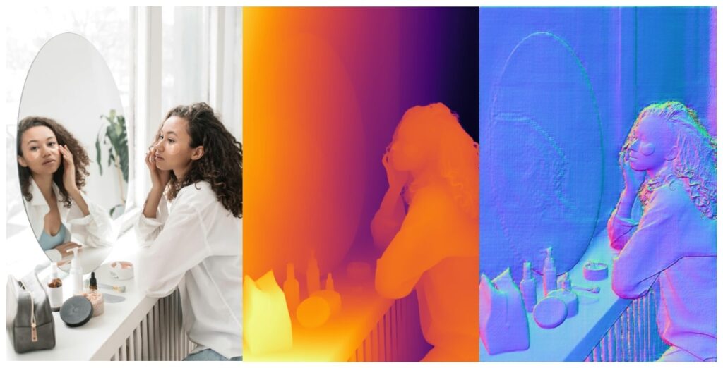
Though, Depth Pro is an impressive, yet it too has failure scenarios such as blurred objects and foggy conditions, where it fails to get any meaningful results of subjects beyond the haze, While the structures of these subjects become slightly visible when surface normals are computed, however they are not apparent to a naked eye in the inverse or raw depth map. Sometimes, it does infer the reflections in the mirror as real humans which isn’t desirable.
1. Blurred Subjects
2. Foggy Scene
3. Mirror Reflections
4. Graffiti Illusions
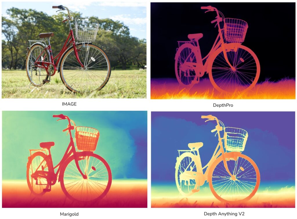
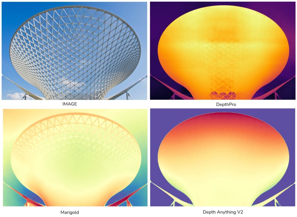
Comparison 1: Image Inference – Depth Pro v/s Depth Anything V2 v/s Marigold
Compared to Depth Anything V2, Depth Pro outputs are high-res and sharp where crisp details without any washed out pixels.
Sample 1
Sample 2
Comparison 2: Video Inference – Depth Pro v/s DepthCrafter
Depth Pro doesn’t support native video depth, so we will split the video as frames and pass the dir containing all frames to Depth Pro. On the other hand, Tencent’s DepthCrafter is an SOTA video depth model, which employs an image-to-video diffusion model internally. As a result from the following set of comparison between samples, we can clearly see that DepthCrafter produces consistent depth for these high motion and dynamic videos, whereas depth pro struggles in handling these scenarios producing flickering or washed-out depth maps. This emphasizes the importance of accounting temporal information into the context for generating coherent depth maps.
Sample 1
Sample 2
Applications with Depth Pro’s Depth Map
Have you ever thought about how Meta 3D photo sharing features in their social platforms work? It uses image depth data to create those effects. Similarly, portrait mode on Pixel or iPhones saves depth data, enabling realistic 3D styles and effects. While depth maps have numerous applications in autonomous driving, medical imaging, gaming/XR, 3D reconstruction, and robotics, in this article, we’ll focus on some of their uses in photo and video editing at a high level.
Application 1: Parallax Effect with Adobe Software
Photoshop by default has a relative depth based depth blur model named bottlenet in its neural filter plugins, which comes in handy when adding movement to static images.
Instead of using the default plugin’s output, we imported DepthPro’s raw depth map into the project and applied it to the input to create a parallax effect with After Effects.

Application 2: Simulating Depth of Field Effect from Static Image
To simulate the focal properties of a real camera, all you have to do is the depth map. Depth of Field creates sharp focus on the focal plane at a specific distance, while keeping all other areas blurred. It refers to the distance between the nearest and farthest objects that appear acceptably sharp in an image.
rgb_image = cv2.resize(rgb_image, (new_width, new_height))
depth_map_normalized = cv2.resize(depth_map_normalized, (new_width, new_height))

# Function to apply depth of field effect
def apply_dof(focal_depth):
   focal_range = 0.1  # Range around focal depth to remain sharp

   # Create smooth focus weights
   sharpness_weights = np.exp(-((depth_map_normalized - focal_depth) ** 2) / (2 * focal_range ** 2))
   sharpness_weights = sharpness_weights.astype(np.float32)

   # Apply Gaussian blur to the background
   blurred_image = cv2.GaussianBlur(rgb_image, (51, 51), 0)

   # Blend the original image and blurred image using sharpness weights
   sharpness_weights_3d = np.expand_dims(sharpness_weights, axis=2)  # Add a channel for blending
   dof_image = sharpness_weights_3d * rgb_image + (1 - sharpness_weights_3d) * blurred_image
   dof_image = np.clip(dof_image, 0, 255).astype(np.uint8)
   return dof_image

# Callback function for the trackbar
def on_trackbar(val):
   # Convert slider value (0-100) to focal depth (0.0-1.0)
   focal_depth = val / 100.0
   dof_image = apply_dof(focal_depth)
   cv2.imshow("Depth of Field Effect", dof_image)

# Create a window and resize it to fit the screen
cv2.namedWindow("Depth of Field Effect", cv2.WINDOW_NORMAL)
cv2.resizeWindow("Depth of Field Effect", new_width, new_height)

# Create a trackbar (slider) at the top of the window
cv2.createTrackbar("Focal Plane", "Depth of Field Effect", 50, 100, on_trackbar)  # Default at middle (50)

# Show initial DOF effect
initial_dof_image = apply_dof(0.5)  # Start with focal depth at 0.5
cv2.imshow("Depth of Field Effect", initial_dof_image)
Application 3: Depth Blur / Portrait Mode
One of the real application were depth data is extremely useful is in getting cool portrait effect in mobile camera’s where they have fixed focal length unlike DSLR lens with varying focal length.
# Normalize depth map to range [0, 1]
depth_map_normalized = cv2.normalize(depth_map.astype(np.float32), None, 0, 1, cv2.NORM_MINMAX)

# Convert normalized depth map back to uint8 (0-255 range)
depth_map_uint8 = (depth_map_normalized * 255).astype(np.uint8)

# Automatically infer focus range
min_depth = np.min(depth_map_normalized)
focus_margin = 0.22  # start with 10% margin for focus range -> 0.1
focus_near = int(min_depth * 255)
focus_far = int((min_depth + focus_margin) * 255)

# Debug: Print focus range
print(f"Focus range: {focus_near} to {focus_far}")

# Create a binary mask for the focus region
focus_mask = cv2.inRange(depth_map_uint8, focus_near, focus_far)

# Apply Gaussian blur to the entire image
blurred_image = cv2.GaussianBlur(rgb_image, (51, 51), 0)

# Convert focus mask to 3 channels for blending
focus_mask_color = cv2.merge([focus_mask, focus_mask, focus_mask])

# Blend images: Keep original where mask is white, blur otherwise
result = np.where(focus_mask_color == 255, rgb_image, blurred_image)

# Save and display the result
cv2.imshow("Depth Blur Effect", result)

Application 4: 3D Point Cloud Projection from Depth Map
Finally, we will explore a common application of creating 3D point clouds from 2D images using depth maps.
Metric depth has an edge over relative depth estimates when a pixel is projected into 3D space. Unlike relative depth models, metric depth allows scaling with the help of field of view, calculated by formula, f_px / image width.
The following code block generates point clouds and reprojects into 3D using Open3D visualization toolkit.
focal_length_x  = 140 #In mm
focal_length_y = 140 #In mm

x,y = np.meshgrid(np.arange(width), np.arange(height))

x = (x - width /2) / focal_length_x
y = (y - height / 2) / focal_length_y

z = np.array(depth_raw)

points = np.stack((np.multiply(x,z), np.multiply(y, z), z), axis = -1).reshape(-1, 3)
colors = np.array(color_img).reshape(-1, 3) / 255.0

# Create the point cloud and save it to the output directory
out_dir = "Applications/vis_point_cloud"
os.makedirs(out_dir, exist_ok=True)
pcd = o3d.geometry.PointCloud()

pcd.points = o3d.utility.Vector3dVector(points)
pcd.colors = o3d.utility.Vector3dVector(colors)

o3d.io.write_point_cloud(f'{os.path.join(out_dir, "satya.ply")}', pcd)

# Load in the point cloud created from OpenCV to compared to Open3D
opencv_pcd_path = "Applications/vis_point_cloud/satya.ply"
pcd = o3d.io.read_point_cloud(opencv_pcd_path)

# Flip it, otherwise the pointcloud will be upside down
pcd.transform([[1, 0, 0, 0], [0, -1, 0, 0], [0, 0, -1, 0], [0, 0, 0, 1]])
o3d.visualization.draw_geometries([pcd])
The outputs aren’t great, and we may need to fix camera intrinsics in the reprojection matrix. However using the image metadata, we were able to get the focal length as 70-200mm@140mm with F/4.5. By using that f_px and performing transforms with Q matrix (reprojection), this is the best possible point cloud we have obtained.
Key Takeaways from Depth Pro
- Depth Pro is faster and produces higher resolution depth maps with an effective training strategy. Compared to other monocular depth estimators, depth pro’s output is crisp and features sharp boundaries.
- We have shown a cherry-picked demo for inferring distance from the depth map with two cases (card board). However we faced discrepancies in getting expected distance when we tried with other examples. Let us know in the comments, if you have a right pipeline with logic that handles it correctly.
- We strongly believe Depth Pro is another feather to the monocular depth field, after MiDaS and DepthAnything’s legacy. However it is limited by the absence of an official fine-tuning pipeline and is licensed under Apple with special clauses for broader adoption.
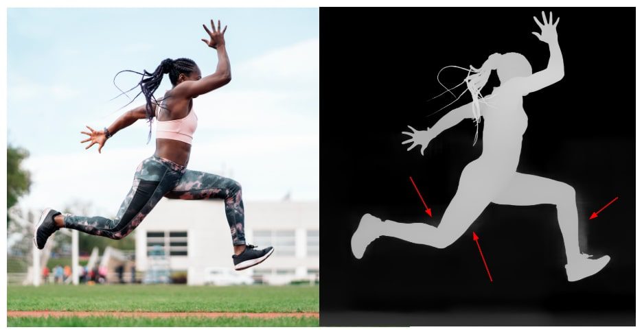
- Despite its advancements, Depth Pro faces challenges such as “flying pixels” or artifacts in depth maps that can distort images and boundary tracing issues. However, it performs better than previous models in these areas.
Conclusion
What do you think about Depth Pro results? Quite impressive, isn’t it? As Depth Pro is a foundational model it can be extended to other downstream tasks like Novel view synthesis, surface normal estimation, semantic segmentation, depth completion, 3D Reconstruction etc., It would have been a great addition to open source community if the project was licensed under a MiT or Apache 2.0. If you are planning to use the model for commercial purpose be sure to check the licensing clause.
For this article, working along with our media team, for ideation, particularly to understand the cross functional application of computer vision especially depth in softwares like Adobe Photoshop and After Effects for content creation, helped to gain a lot of hindsight. What interesting applications you have built with depth map? Let us know in comments, we would love to hear them.
References
2. Interesting Read by PatricioGonzalez
3. HuggingFace: Monocular depth estimation guide
4. Surface normal from depth code snippet: Decoding Meta Sapiens
5. DepthAnything V2 : Metric Depth
6. Open3D Tutorials by Nicolai Neilsen


