In the groundbreaking 2017 paper “Attention Is All You Need”, Vaswani et al. introduced Sinusoidal Position Embeddings to help Transformers encode positional information, without recurrence or convolution. This elegant, non-learned mechanism uses sine and cosine functions to encode token positions in a way that generalizes beyond fixed sequence lengths.
The blog post provides a comprehensive examination of Sinusoidal Position Embeddings, exploring their functionality, rationale for selection, comparison with alternatives, and the insights gained from experiments on their behavior.
- Why Positional Embeddings Are Needed
- Origins of Sinusoidal Position Embeddings
- Mathematical Formula Explained
- Intuition Behind the Design
- Code to generate Sinusoidal Position Embeddings
- Sinusoidal Embeddings: What They Enable
- Differentiating Rotary and Sinusoidal Position Embeddings
- Why This Helped Transformers Before RoPE
- Conclusion
- References
Why Positional Embeddings Are Needed
The first implementation of positional encoding was the sinusoidal method, introduced by the original Transformer paper in 2017. The authors proposed a non-learned, deterministic approach using sine and cosine functions of varying wavelengths.
Their key motivation: create a position representation that enables generalization to longer sequences than those seen during training.
Origins of Sinusoidal Position Embeddings
The first implementation of positional encoding was the sinusoidal method, introduced by the original Transformer paper in 2017. The authors proposed a non-learned, deterministic approach using sine and cosine functions of varying wavelengths.
Their key motivation: create a position representation that enables generalization to longer sequences than those seen during training.
Mathematical Formula Explained
The sinusoidal position embedding PE for a token at position pospospos with embedding dimension i is defined as:
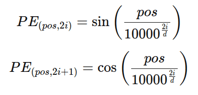
- pos: Token index in the sequence
- i: Index in the embedding vector
- d: Dimensionality of the embedding space
This alternating pattern ensures different frequencies across dimensions.
Intuition Behind the Design
Why sine and cosine? Here’s the reasoning:
- Smooth and Periodic: Allows nearby positions to have similar vectors.
- Frequency Bands: Embeddings capture both coarse and fine positional changes.
- Relative Position Inference: The Distance between two positions can be approximated from the inner product of their encodings.
- No Parameters to Train: Reduces overfitting risk and memory usage.
Key Insight:
This design is similar to how the Fourier basis decomposes functions. Lower dimensions capture slower changes (global patterns), higher dimensions capture faster oscillations (local details).
Code to generate Sinusoidal Position Embeddings
Here’s a complete walkthrough and explanation of the way sinusoidal position embeddings are being generated from an input sentence –
def get_sinusoidal_embeddings(seq_len, d_model):
    position = np.arange(seq_len)[:, np.newaxis]
    print(position)
    div_term = np.exp(np.arange(0, d_model, 2) * -np.log(10000.0) / d_model)
    print(div_term)

    embeddings = np.zeros((seq_len, d_model))
    embeddings[:, 0::2] = np.sin(position * div_term)
    embeddings[:, 1::2] = np.cos(position * div_term)

    return embeddings
Explanation –
position = np.arange(seq_len)[:, np.newaxis]
np.arange(seq_len)– Creates a vector[0, 1, 2, ..., seq_len-1]– one for each token position.- The
[:, np.newaxis]converts it from shape(seq_len,)to(seq_len, 1)for broadcasting in matrix operations.
—> This assigns a unique position index to each row.
div_term = np.exp(np.arange(0, d_model, 2) * -np.log(10000.0) / d_model)
This creates the divisor term used in the sinusoidal formula:

Let’s unpack it:
np.arange(0, d_model, 2)→ indices[0, 2, 4, ..., d_model-2]for even positions in the embedding vector.- Each index
icorresponds to a frequency band. - The exponential term produces the
div_termcorresponding to each position i used in the sinusoidal formula –

—> This term controls how fast each sinusoidal dimension oscillates.
embeddings = np.zeros((seq_len, d_model))
- Creates an empty embedding matrix of shape
(sequence_length × embedding_dim) - Each row represents a position in the sequence, and each column represents a dimension of the embedding vector.
embeddings[:, 0::2] = np.sin(position * div_term)
0::2slices all even dimensions in the embedding vector.- The broadcasting
position * div_termresults in a matrix where each element is:

- This fills even-indexed dimensions with sine curves of increasing frequency.
embeddings[:, 1::2] = np.cos(position * div_term)
1::2slices all odd dimensions.- Same multiplication, but with
cosinstead ofsin.
—> Alternating sine and cosine curves across dimensions.
So What’s Happening Conceptually?
Each token gets a vector:

Where each frequency

This structure means:
- Low dimensions change slowly (global position features)
- High dimensions change rapidly (local position features)
This allows attention layers to:
- Use dot products between embeddings to estimate relative distances
- Encode both local and long-range ordering without recurrence
| Dimension | Behavior | Interpretation |
|---|---|---|
| 0–1 | Slow oscillation | Capture broad/global positions |
| 6–7 | Fast oscillation | Capture fine/local positional changes |
| All | Orthogonal frequency patterns | Unique positional signature per token |
| Together | Smooth, continuous combination | Multi-resolution encoding of position |
Visualizing Sinusoidal Embeddings
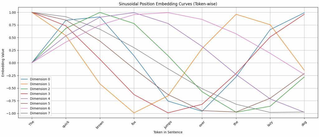
The above plot illustrates the sinusoidal position embeddings for the sentence “The quick brown fox jumps over the lazy dog.” Each colored line represents one of the first 8 dimensions of the positional embedding vector, showing how its value changes across token positions. Lower dimensions oscillate slowly, capturing broad positional trends, while higher dimensions fluctuate more rapidly, encoding finer positional distinctions. Together, these multi-frequency sinusoidal curves uniquely encode each token’s position and provide the Transformer with a mathematically structured sense of order.
Sinusoidal Embeddings: What They Enable
Inject Token Order into Input
By adding these sinusoidal vectors to the token embeddings:
final_embedding = word_embedding + position_embedding
…each token now carries information about both its content and position.
Relative Distance Awareness
Even though sinusoidal embeddings are absolute, their inner product behavior enables relative comparisons:
- The dot product of position vectors
PE(pos1)⋅PE(pos2)reflects the distance between tokens. - This helps attention mechanisms favor nearby tokens or model long-distance relationships depending on the task.
Generalization Beyond Training Length
- These embeddings are generated by a formula, not learned weights.
- That means a model trained on length 100 sequences can still handle length 200 during inference – just compute sinusoidal encodings for more positions.
This wouldn’t be possible with learned position embeddings, which are limited to training-time max length.
Multi-Scale Awareness
Lower dimensions: slow sinusoidal change → global structure
Higher dimensions: rapid change → precise token index encoding
Together, the full vector allows attention heads to capture both local (e.g., “brown fox”) and global (e.g., sentence structure) relationships.
Differentiating Rotary and Sinusoidal Position Embeddings
A common misconception is that Rotary Position Embeddings (RoPE) and Sinusoidal Position Embeddings operate the same way because both rely on sine and cosine functions. However, they are fundamentally different in where and how they encode position.
While Sinusoidal Position Embeddings are absolute and additive, directly added to token embeddings before attention, RoPE is relative and multiplicative, applied during the attention calculation itself. RoPE rotates the query and key vectors in a shared phase space so that relative positional information emerges directly in the attention scores.
Conceptual Differences
Sinusoidal Embeddings (Absolute + Additive)
- Precomputed vector of sin/cos values per position.
- Added directly to the token embedding: “
Input Embedding = Token Embedding + Position Embedding“ - Attention then operates on these modified inputs.
- Positional information is baked into the token — all downstream layers rely on this.
Rotary Embeddings (Relative + Multiplicative)
- Instead of adding, it applies a rotation matrix to the query and key vectors before the dot-product attention:

- The rotation encodes position-dependent phase shifts.
- These phase shifts encode relative distances directly into the attention scores.
Intuition: Rotation vs Addition
Imagine each token embedding as a vector in space:
- Sinusoidal embeddings shift each token by a fixed vector (added position)
- RoPE rotates the token in space, creating a directional signal tied to position
Because the dot product between two rotated vectors reflects their relative distance, RoPE gives native access to relative position without learning or storing extra embeddings.
Why This Helped Transformers Before RoPE
Before rotary embeddings or learned relative ones, sinusoidal embeddings gave Transformers:
- A simple way to inject position without training more parameters
- The ability to extrapolate to unseen sequence lengths
- A natural method to approximate token distances through phase differences
And because attention works via dot products between vectors, the phase alignment of sinusoidal vectors becomes mathematically meaningful, enabling models to learn ordering patterns without explicitly learning them.
Conclusion
Sinusoidal Position Embeddings remain a foundational concept in Transformer architectures. They demonstrate that elegant mathematical formulations can compete with and even outperform learnable alternatives in certain contexts.
Their smooth generalization, zero-parameter nature, and interpretable structure make them ideal for:
- Research prototyping
- Edge devices
- Models needing extrapolation to longer sequences
As Transformer architectures continue to evolve, sinusoidal embeddings remind us that sometimes simplicity is powerful.





100K+ Learners
Join Free OpenCV Bootcamp3 Hours of Learning