Self-attention, the beating heart of Transformer architectures, treats its input as an unordered set. That mathematical elegance is also a curse: without extra signals, the model has no idea which token, word, or patch is first, second, or adjacent. Position embeddings solve this by injecting a “sense of order,” allowing language models to form coherent sentences and Vision Transformers to respect spatial layouts. We can think of it as an extra vector added to every token that acts like a coordinate tag.
Position embeddings are the quiet backbone of every modern Transformer. From the first sinusoidal vectors in 2017 to today’s rotary, bias-based, and Fourier encodings, each breakthrough has balanced parallelism, relative distance awareness, and context length. RoPE sits at the sweet spot: elegant math, zero extra parameters, and scalability proven in the largest LLMs in production. Understanding its clocks, scaling tricks, and edge cases is now essential engineering lore for anyone building or fine-tuning state-of-the-art language or vision models.
- From Recurrence to Explicit Coordinates
- Historical Origins – Where Did Position Embeddings Come From?
- Absolute Position Embeddings (The First Generation)
- Relative Position Embeddings (Second Generation)
- Bridging the Gap: Rotary Position Embeddings (RoPE)
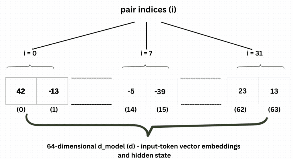
- The role of d (d_model) in a Transformer and in RoPE
- How different pair indices (i) serve different roles
- Visualizing RoPE Implementation
- RoPE Implementation Code
- Visualisation Code and Case Studies
- d_model d = 64, pair_index i = 0 and input sequence length = 6
- d_model d = 64, pair_index i = 7 and input sequence length = 6
- d_model d = 64, pair_index i = 7 and input sequence length = 47
- d_model d = 1024, pair_index i = 87 and input sequence length = 30
- d_model d = 1024, pair_index i = 87 and input sequence length = 32
- Why this isn’t a hard “context limit”
- Rule-of-thumb formula to calculate Tmax in RoPE Clocks with specific d
- Powerful Insights
- What does make RoPE performance drop at long context
- Other positional issues RoPE can’t solve
- Conclusion
- References
From Recurrence to Explicit Coordinates
| Architecture | How did it know the order | Bottleneck |
|---|---|---|
| RNN/LSTM | Time-step recursion = built-in index | Slow, gradient decay |
| CNN (ByteNet, WaveNet) | Convolution stride/dilation = distance | Many layers for long context |
| Transformer (2017) | Introduced sinusoidal absolute PE | Needs explicit coordinates |
The sinusoid scheme added sin and cos waves of geometric wavelengths directly to token vectors, letting the network infer relative offsets by linear combination. It was simple, parameter-free, and the starting point for everything that followed.
Historical Origins – Where Did Position Embeddings Come From?
| Year | Milestone | Why It Mattered |
|---|---|---|
| 2017 | Attention Is All You Need introduces absolute sinusoidal position encodings. | Gave the very first Transformer a way to model sequence order without recurrent nets. |
| 2018 | Shaw et al. propose learned relative position embeddings. | Showed that distance, not fixed position, is often what models truly need. |
| 2019 | Transformer-XL generalizes relative encodings to very long contexts. | Enabled language models to handle thousands of tokens without architectural change. |
| 2021 | Rotary Position Embedding (RoPE) (Su et al., RoFormer) elegantly fuses distance awareness into the dot-product itself. | Became the default in Llama, Qwen, Gemma, and many vision-language models. |
Absolute encodings appeared first, baked into the original Transformer; relative approaches were invented a year later, inspired by limitations seen in longer sequences.
Absolute Position Embeddings (The First Generation)
What Are They?
A vector e is assigned to each position of the input. It is added to the token embedding before the first attention layer:

Why Sinusoidal Position Embeddings?
- Continuous and differentiable – helpful for optimization.
- Each frequency captures a different “granularity” of position (token-level vs clause-level).
- The phase difference between two positions is a linear function of distance, enabling the model to decode relative offsets algebraically.
Two Popular Flavors
| Variant | Construction | Strengths | Weaknesses |
|---|---|---|---|
| Learned Lookup Table | Train a unique vector per position. | Task-specific bias; fastest to implement. | Hard upper limit on max length; can’t extrapolate. |
| Sinusoidal Encoding (original paper) | Fixed, parameter-free sin-cos waves at log-scaled frequencies. | Zero extra params; mildly extrapolates to unseen lengths by mathematical design. | Can’t adapt to task biases; still “absolute”. |
Drawbacks associated with Absolute Position Embeddings
Absolute (sinusoidal) PEs solved the permutation-invariance problem but left distance reasoning, long-context stability, and caching efficiency to chance. Relative approaches, including Shaw-18 bias, T5 buckets, ALiBi, and RoPE, make distance explicit, scale length gracefully, and simplify state reuse, which is why they displaced pure absolute encodings in today’s high-performing LLMs.
Relative Position Embeddings (Second Generation)
Motivating Shift
For language and music, distance (“how far apart”) is more informative than absolute index (“position 42”). Relative schemes inject a bias into the attention score between tokens i and j:

where the bias b depends only on the offset (i-j), so the network gets “token right next to me” vs. “token 50 steps back” for free.
Design Variants
| Approach | Key Idea | Notable Implementations |
|---|---|---|
| Additive Distance Embeddings | Learn a vector per offset, add to q or k. | Self-Attention with Relative Position Representations Paper |
| Transformer-XL Bias | Shares parameters across segments to unroll histories. | Transformer-XL, XLNet |
| Bucketed Relative Bias | Group distances into logarithmic “buckets”. | T5, DeBERTa |
| ALiBi (Attention with Linear Biases) | Adds a slope × distance term – zero new tensors, constant memory. | GPT-NeoX-20B, long-context LLMs |
| CABLE / GLiN (2024-25) | Context-aware learnable functions of distance. | Research prototypes for 100-k-token windows |
Benefits over Absolute Schemes
- Extrapolation: Works seamlessly for longer sequences.
- Parameter Efficiency: Same embedding reused across all positions.
- Inductive Bias: Captures translation invariance (useful for both text and images).
Drawbacks associated with Relative Position Embeddings
Early RPEs made distance explicit but paid for it with tables, buckets, and runtime gather ops.
RoPE delivers the same distance signal by converting position into a phase rotation – an analytical, continuous, and parameter-free approach – allowing it to scale to large contexts and integrate seamlessly into fast attention kernels.
Bridging the Gap: Rotary Position Embeddings (RoPE)
The Rotational Trick
RoPE stores position as a rotation in each even/odd dimension pair:
![RoPE Theta Rotation Formula – LearnOpenCV A formula block showing the core Rotary Position Embedding math. Left: θₚ,ᵢ = p / 10000^(2 i / d), where p is the token index, i the pair index, and d the model dimension. Right: the 2×2 rotation matrix R(θ) = [[cos θ, –sin θ], [sin θ, cos θ]], indicating how each even–odd dimension pair is rotated by angle θ.](https://learnopencv.com/wp-content/uploads/2025/07/RoPE-Theta-Rotation-Formula.png)
Queries and keys are rotated by R(θp,i). The dot-product becomes a function of (θp,i−θq,i) ∝ distance (p−q), so distance, not absolute index, drives attention. In simple terms, RoPE rotates query and key vectors in a shared 2-D sub-space by an angle proportional to their positions. After rotation, their dot product encodes only the relative distance. It merges the mathematical elegance of sinusoids with the distance focus of relative bias – no extra tables, and the rotation is computed on the fly.
Hidden States / Hidden Dimensions in a Transformer
Every token inside a Transformer layer is represented by a vector of length d (often called d_model or d_head after it is split across heads).
Think of that vector as a slot rack of d numbers that can store:
| part of the vector | can learn to carry … |
|---|---|
| lower few dims | lexical identity (“this looks like cat”) |
| middle dims | syntactic role (“subject noun”) |
| higher dims | long-range features (“begins a quotation”) |
The larger d is, the more distinct patterns the model can encode, at the cost of larger weight matrices (compute ↑, memory ↑).
What sits inside each pair during training
During forward pass:
- Input token → linear layer → raw query/key vectors.
- Apply RoPE rotation per pair for each vector.
- Feed those into dot-product attention.
During gradient updates, the network learns weight patterns so that certain directions in those 2-D sub-spaces fire for meaningful distances (e.g., “two tokens back” for a bigram pattern) because Δθ appears multiplicatively inside the attention logit formula.
Connecting back to Self-attention
Inside the Transformer layer, our rotated queries/keys produce an attention weight:

- In RoPE, each position ppp in a sequence is assigned an angle θp based on its position index and the pair index iii (which corresponds to a 2-D slice in the model’s hidden dimension). When computing the attention between two tokens, the difference in the angles of two positions p and q is what actually matters. This relative difference Δθ between tokens p and q is proportional to their positional distance. The model does not need to know absolute positions but instead learns the relative distance between positions.
- The network can thus learn distance-aware patterns (e.g., “Look two tokens back if current token is a verb”) without an explicit relative-position table.
That is exactly what makes RoPE the default positional strategy in Llama-2/3, Gemma, Mistral, Code-Llama (with NTK scaling), YaRN, etc.
Why It’s Powerful
- Relative by construction: no lookup tables.
- Parameter-free: weight count identical to absolute sinusoids.
- Smooth extrapolation: angles extend indefinitely; with NTK/YaRN scaling, they remain stable to 256k+ tokens.
- Streaming-friendly: rotation is done once when writing the KV cache.
The role of d in a Transformer and in RoPE
| Symbol | In the code/paper | What it controls |
|---|---|---|
d (often called d_model) | Length of every token-embedding vector & hidden state (e.g., 64 in our plots, 4,096 in Llama-3-8B) | • Model capacity – more dimensions ⇒ larger weight matrices, more parameters, higher compute/memory cost. • Number of position “channels” available to RoPE (each channel = one cos + sin pair, so there are d / 2 of them). |
Why d must be even for RoPE
RoPE divides the vector into 2-D slices.
For every slice, it computes

and rotates the corresponding query and key components.
If d were odd, we would end up with a leftover single dimension that can’t form a cosine/sine pair, so practical implementations either:
- choose
dto be even (the usual solution), or - drop/pad one dimension after projection to the per-head size
d/h.
What more dimensions buy us in RoPE
Because RoPE uses a geometric progression of frequencies

i = 0(first pair) → fastest “clock” (1 rad per token in our plots).- Higher
i→ progressively slower clocks (longer wavelengths).
Increasing d therefore:
- Adds more clocks: we get
d / 2of them instead of, say,32 / 2 = 16. - Fills in frequency gaps more finely: the exponent step
2/dbecomes smaller, so the model sees a smoother spectrum of time scales, helpful for picking up subtle relative offsets.
Downstream consequences of choosing d
| Design lever | Effect |
|---|---|
Larger d | ↑ Parameter count (weights are d×d); ↑ FLOPs per token; ↑ memory. Improved capacity to model fine-grained dependencies; more RoPE channels, potentially leading to better long-context performance. |
Smaller d | ↓ Compute & memory (good for mobile / edge). But fewer channels ⇒ less expressive position signal and lower model capacity. |
Per-head dimension (d/h) | Each attention head sees its own slice of the data. All slices must still be even so every head can apply RoPE locally. |
Why RoPE still helps at any reasonable d
Even with modest dimensions (e.g. d = 128 = 64 pairs), RoPE already provides:
- Relative encoding (attention depends on p–q, not absolute indices).
- Parameter-free operation (no extra learned table).
- Smooth extrapolation beyond the training window, because those sines/cosines extend indefinitely.
Hence, modern LLMs pick d primarily for model capacity and hardware efficiency, but RoPE will dutifully scale along, giving each additional dimension a fresh positional “clock” for the network to exploit.
How different pair indices (i) serve different roles
Pair index i (0 → slowest) | Wavelength (tokens/lap) when d = 1024 | Typical use in the network |
|---|---|---|
| 0–3 (fast) | Wavelength (tokens/lap) when d = 1024 | Local n-grams, word morphology, punctuation. |
| 4–50 | 20 – 200 | Phrase & sentence syntax, within-paragraph cohesion. |
| 50–200 | 200 – 5,000 | Cross-paragraph references, code-block scopes, doc sections. |
| 200–511 (very slow) | 5,000 – 62,000 | Chapter-level, entire-file context; acts almost like a “segment ID”. |
Visualizing RoPE Implementation
RoPE Implementation
Configuration block
d =  1024         # hidden (or head) size, must be even
pair_idx = 87     # the (cos,sin) pair to plot
dis the per-head hidden width.
RoPE requires an even size so each adjacent pair of dimensions can hold a cosine + sine.
pair_idx= i chooses which 2-D slice of the d-vector we visualise.
Tokenisation & absolute positions
tokens = paragraph.split()
p = np.arange(len(tokens))      # positions 0,1,2…
This mimics the positional index p that the real model would feed into the RoPE formula.
RoPE angle schedule
base   = 10000 ** (2*pair_idx / d)
angles = p / base
Exactly the analytic rule from RoPE’s paper:

2*pair_idx/dis the exponent.baseis therefore 10000^{2i/d}.anglesis the vector of θp,i for every token.
This is the core RoPE computation: no learning, just deterministic geometry.
Map angles to a 2-D vector
x, y = np.cos(angles), np.sin(angles)
For the chosen pair, RoPE stores [cosθp,i, sinθp,i] into dimensions (2i, 2i + 1) of the token’s 1024-D hidden state. Plotting (x, y) shows how that slice rotates as p grows.
Visualisation and Case Studies
plt.figure(figsize=(6, 6))
plt.scatter(x, y, marker="x")

# Dotted rays with token labels mid-way
for xi, yi, tok in zip(x, y, tokens):
    plt.plot([0, xi], [0, yi], ":", lw=1)
    plt.text(0.6*xi, 0.6*yi, tok, ha="center", va="center")

# Unit circle and grid
plt.gca().add_artist(plt.Circle((0, 0), 1, fill=False, ls="--"))
plt.grid(ls="--", lw=0.4, alpha=0.4)

plt.title(f"RoPE pair {pair_idx} of d={d} (dim {2*pair_idx}/{2*pair_idx+1})")
plt.xlabel("cos θ"); plt.ylabel("sin θ")
plt.axis("equal"); plt.show()
- Each cross = one token’s 2-D projection.
- Dotted ray illustrates the rotation matrix that will later be applied to that token’s query/key components.
Unit circle + grid reinforce that every point has magnitude 1 (a property RoPE needs to keep vector norms intact).
How does this reflect “real” RoPE internals
| In the code | Inside a Transformer layer |
|---|---|
Compute angles | During forward pass, the same θ is computed (or cached) for each sequence length. |
Take cos, sin | Those values form either (a) an explicit position vector concatenated to token states, or (b) the rotation matrix applied to Q, K. |
| Visualise one pair | The model holds 512 pairs; attention utilizes all of them, resulting in a high-dimensional full position signature. |
Rays but no rotation of Q,K | In the real kernel, Qp and Kp are multiplied by R(θp,i), that’s the only missing step here. |
Let’s understand the role of d (d_model or dimension) and pair_index (i) in RoPE with some case studies.
d_model d = 64, pair_index i = 0 and input sequence length = 6
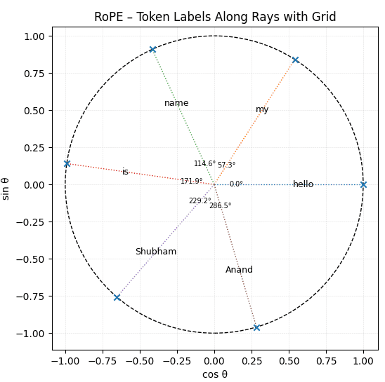
What the picture is actually showing
- Each point = one token from our sentence.
- The axes are
cos θ(-1 → +1) andsin θ(-1 → +1). - For i = 0, angles calculation is as follows –
| position p | angle θp | in degrees |
|---|---|---|
| 0 | 0 rad | 0 ° |
| 1 | 1 rad | 57.3 ° |
| 2 | 2 rad | 114.6 ° |
| 3 | 3 rad | 171.9 ° |
| 4 | 4 rad | 229.2 ° |
| 5 | 5 rad | 286.5 ° |
- A full lap needs 2π ≈ 6.283 rad.
- After five steps, we have covered only 5rad ≈ 286.5°, so “Anand” is still 73.5 ° short of meeting “hello”.
- If we had added a seventh token, its angle would be θ6 = 6rad ≈ 343.8°; only after the eighth token (θ7 ≈ 401.1° ≈ 360° + 41.1°) would the clock pass the starting point.
d_model d = 64, pair_index i = 7 and input sequence length = 6
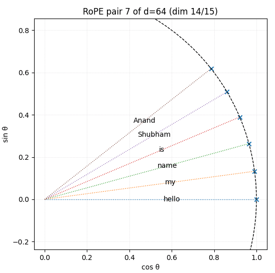
Why do the rays barely rotate
With d = 64 and i = 7, we get –

| token | position p | θ (rad) | θ (°) |
|---|---|---|---|
| hello | 0 | 0.000 | 0° |
| my | 1 | 0.133 | 7.6° |
| name | 2 | 0.267 | 15.3° |
| is | 3 | 0.400 | 22.9° |
| Shubham | 4 | 0.533 | 30.5° |
| Anand | 5 | 0.667 | 38.2° |
A full revolution (2π ≈ 6.283 rad) now requires approximately 47 tokens if we divide 2π by 0.133. Let’s verify that we’re going in the right direction by providing the input length as 47.
d_model d = 64, pair_index i = 7 and input sequence length = 47
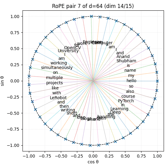
As can be inferred from the above image, exactly 47 tokens fit into a single lap of the circle generated from the 8th pair of the vector embeddings of each token present in the corpus.
Why does the model need these slow clocks?
- Pair 0 wrapped after ~6 tokens; by token 50, it has spun eight times, ambiguous by itself.
- Pair 7 won’t wrap until token 47; pair 31 (the slowest) needs ~50,000 tokens!
Because attention uses all 32 clocks simultaneously, two positions collide only if they share the same phase in every pair… which doesn’t happen until we surpass the longest wavelength.
d_model d = 1024, pair_index i = 87, and input sequence length = 30
Now, according to our calculation, for d = 1024, a rotation period of almost 30 tokens requires a pair index of 87. Let’s verify our calculation approach –
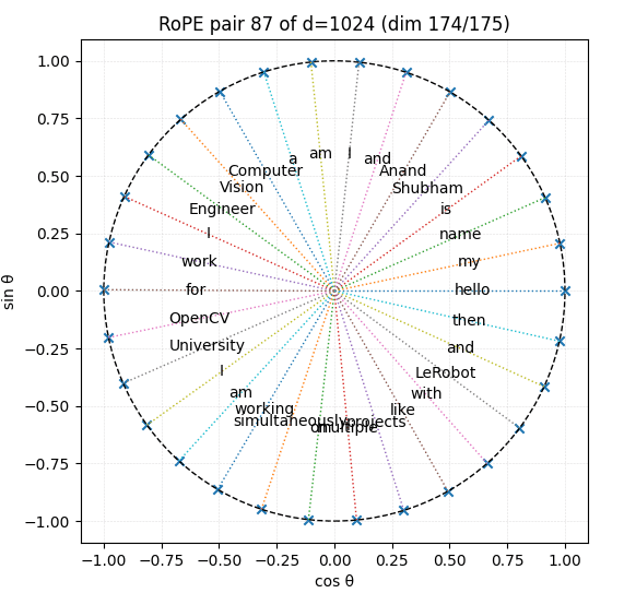
So yes, pair_index 87 with dimensions (174/175) along with 30 tokens as input length, will complete one rotation.
d_model d = 1024, pair_index i = 87 and input sequence length = 32
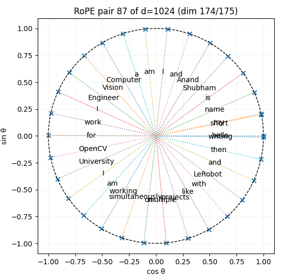
As can be inferred from the above graph, for pair_index 87 and d = 1024, input sequence length exceeding 30 tokens starts getting wrapped.
With RoPE and a per-head width d = 1024 , the slowest clock (pair 511) makes one full revolution after ≈ 6.2 × 10⁴ tokens, roughly sixty-one thousand tokens.
Why this isn’t a hard “context limit” in RoPE
- Every head has
d/2 = 512clocks.
A token pair aliases only if all 512 phases align again, which happens far beyond 61k tokens (their periods are incommensurate).
- Large LLMs still need attention, memory, and numerical stability tricks (NTK, YaRN, sliding-window, etc.) to push context to 128k–1M tokens, but the RoPE spectrum itself keeps phase collisions extremely rare up to roughly the slowest-clock period.
- So Tmax is best seen as the largest single-clock wavelength; overall uniqueness persists orders of magnitude farther.
Rule-of-thumb formula to calculate Tmax in RoPE Clocks with specific d

d | slowest-clock lap |
|---|---|
| 64 | 2π⋅10000^{0.968} ≈ 5.0 × 10⁴ |
| 128 | 2π⋅10000^{0.984} ≈ 5.7 × 10⁴ |
| 1024 | ≈ 6.2 × 10⁴ |
| 4096 | ≈ 6.3 × 10⁴ (approaches 2π⋅10^{4} as d→∞ |
Even an enormous jump in d – 64 → 1024, only moves the slowest period from 4.7×10^{4} to 6.2×10^{4} tokens (a ≈30 % change). So once d reaches a few hundred, the slowest wavelength plateaus around 6×10^{4} tokens; RoPE’s ability to go further relies on the multifrequency blend, not on stretching this single number.
Powerful Insights
- Real benefit of large
dis more intermediate clocks (hundreds instead of dozens), reducing aliasing and improving long-context generalisation, not stretching the very slowest clock far past ~60k tokens.
- Large “tokens-per-lap” counts provide a stable, slowly-varying coordinate for the whole document, but are not themselves the hard limit of RoPE’s capacity.
- Pair index matters: fast indices handle local syntax; slow indices encode document-scale location. Transformers learn to read whichever subset a task demands.
- Model quality depends more on the mix and scaling of pairs than on squeezing out ever-longer single laps. That’s why modern LLM engineering focuses on NTK/YaRN scaling, sliding-window masks, and head specialisation rather than merely inflating
dto push the 62k ceiling a few tokens higher.
What does make RoPE performance drop at long context
| Failure mode | Root cause | Observable symptom |
|---|---|---|
| Phase-shift drift | Using the original training slope (base = 10,000) on a much longer window causes high-frequency pairs to spin too quickly, making it difficult for attention to maintain fine detail. | Sudden loss of syntactic coherence or repeated text after ~8k–16k tokens. |
| Numerical precision | For very large p, floating-point rounding collapses sin θ ≈ sin(θ+ε), especially in fp16/bfloat16. | Gradient vanishing in fine-tune; attention logits become noisy for far-right tokens. |
| Kernel/cache mismatch | Some Flash-Attention & KV-cache variants implicitly assume angle ≤ π; when scaled to 256 k via RoPE-linear, we violate that bound. | Model emits garbage once the cache slides beyond a few segments. |
| Training–inference distribution gap | Model only saw 4k tokens; at 32k, it has never learned to chain-reason across segments. | Quality degrades smoothly even if positional math is correct. |
| Modal mis-alignment in VLMs | Text RoPE (1-D) reused for image patches (2-D) causes anisotropy. | Model favours horizontal relations; diagonal relations are misattended. |
| Cross-head interference | All heads share identical clock set; certain heads “lock-on” to harmonics, starving others of positional variance. | Sharp head-wise sparsity in attention heat-maps; instability during SFT. |
Other positional issues RoPE can’t solve
- No learned adaptation – Being parameter-free, RoPE can’t specialise to domain-specific structures (e.g., XML trees) the way a learned RPE could.
- Axis coupling in 2-D/3-D inputs – Standard 1-D RoPE treats flattened patch order; we need Axial-RoPE or 2-D RoPE to remove artefacts.
- Streaming constraints – At extremely long contexts, we still pay O(L²) memory/time unless combined with sliding-window masks or memory-computation hybrids (LongLoRA, Ring-Attention).
- Precision cliffs – In mixed-precision inference, large angles lead to sin, cos values that differ by < ε of fp16, effectively collapsing several high-freq clocks to the same vector (“angle saturation”).
RoPE’s practical weak spots come much earlier than its theoretical 62 k-token slow-clock wrap-around. Real issues include phase drift of the fast clocks, floating-point precision, training-window mismatch, and modality-specific geometry. Modern scaling tricks or hybrid encodings tackle those problems directly; simply enlarging d (and thus marginally bumping the slowest wavelength) does little to cure them.
Conclusion
Rotary Position Embedding has emerged as the most practical positional strategy for modern Transformers: it is parameter-free, inherently relative, and scales gracefully from sub-word n-grams to book-length contexts. By encoding each token’s index as a rotation in multiple cosine-sine planes, RoPE lets attention read distance directly from phase differences while adding zero learnable weights – so the same checkpoint can stretch from a 4k-token training window to 100k+ inference with a simple angle-scaling trick.
The few pain points – fast-clock drift at ultra-long lengths, fp16 precision loss, and flattened 1-D bias on 2-D data – are well-understood and readily patched (NTK/YaRN scaling, fp32 trig, 2-D or Axial RoPE). For most language and multimodal workloads in 2025, RoPE delivers the best trade-off of simplicity, efficiency, and length-extrapolation, making it the default positional choice when we need an ordered signal that “just works.”
References
- The Curious Case of Absolute Position Embeddings
- Self-Attention with Relative Position Representations
- Relative Positional Encoding for Transformers with Linear Complexity
- RoFormer: Enhanced Transformer with Rotary Position Embedding
- When Precision Meets Position: BFloat16 Breaks Down RoPE in Long-Context Training







100K+ Learners
Join Free OpenCV Bootcamp3 Hours of Learning