Home
>
Deep Learning
>
Number of Parameters and Tensor Sizes in a Convolutional Neural Network (CNN)

Number of Parameters and Tensor Sizes in a Convolutional Neural Network (CNN)

In this post, we share some formulas for calculating the sizes of tensors (images) and the number of parameters in a layer in a Convolutional Neural Network (CNN). This post does not define basic terminology used in a CNN and assumes you are familiar with them. In this post, the

Deep Learning

In this post, we share some formulas for calculating the sizes of tensors (images) and the number of parameters in a layer in a Convolutional Neural Network (CNN).

This post does not define basic terminology used in a CNN and assumes you are familiar with them. In this post, the word Tensor simply means an image with an arbitrary number of channels.

We will show the calculations using AlexNet as an example. So, here is the architecture of AlexNet for reference.

AlexNet has the following layers

Input: Color images of size 227x227x3. The AlexNet paper mentions the input size of 224×224 but that is a typo in the paper.
Conv-1: The first convolutional layer consists of 96 kernels of size 11×11 applied with a stride of 4 and padding of 0.
MaxPool-1: The maxpool layer following Conv-1 consists of pooling size of 3×3 and stride 2.
Conv-2: The second conv layer consists of 256 kernels of size 5×5 applied with a stride of 1 and padding of 2.
MaxPool-2: The maxpool layer following Conv-2 consists of pooling size of 3×3 and a stride of 2.
Conv-3: The third conv layer consists of 384 kernels of size 3×3 applied with a stride of 1 and padding of 1.
Conv-4: The fourth conv layer has the same structure as the third conv layer. It consists of 384 kernels of size 3×3 applied with a stride of 1 and padding of 1.
Conv-5: The fifth conv layer consists of 256 kernels of size 3×3 applied with a stride of 1 and padding of 1.
MaxPool-3: The maxpool layer following Conv-5 consists of pooling size of 3×3 and a stride of 2.
FC-1: The first fully connected layer has 4096 neurons.
FC-2: The second fully connected layer has 4096 neurons.
FC-3: The third fully connected layer has 1000 neurons.

100K+ Learners
3 Hours of Learning

Join Free OpenCV Bootcamp

15K+ Learners
3 Hours of Learning

Join Free TensorFlow Bootcamp

10K+ Learners
8 Hours of Learning

Join Free PyTorch Bootcamp

Next, we will use the above architecture to explain

How to calculate the tensor size at each stage
How to calculate the total number of parameters in the network

Size of the Output Tensor (Image) of a Conv Layer

Let’s define

$O$ = Size (width) of output image.
$I$ = Size (width) of input image.
$K$ = Size (width) of kernels used in the Conv Layer.
$N$ = Number of kernels.
$S$ = Stride of the convolution operation.
$P$ = Padding.

The size ( $O$ ) of the output image is given by

$O = \frac{I - K + 2P}{S} + 1$

The number of channels in the output image is equal to the number of kernels $N$ .

Example: In AlexNet, the input image is of size 227x227x3. The first convolutional layer has 96 kernels of size 11x11x3. The stride is 4 and padding is 0. Therefore the size of the output image right after the first bank of convolutional layers is

$O = \frac{ 227 - 11 + 2 \times 0 }{4} + 1 = 55$

So, the output image is of size 55x55x96 ( one channel for each kernel ).

We leave it for the reader to verify the sizes of the outputs of the Conv-2, Conv-3, Conv-4 and Conv-5 using the above image as a guide.

Size of Output Tensor (Image) of a MaxPool Layer

Let’s define

$O$ = Size (width) of output image.
$I$ = Size (width) of input image.
$S$ = Stride of the convolution operation.
$P_s$ = Pool size.

The size ( $O$ ) of the output image is given by

$O = \frac{ I - P_s }{S} + 1$

Note that this can be obtained using the formula for the convolution layer by making padding equal to zero and keeping $P_s$ same as the kernel size. But unlike the convolution layer, the number of channels in the maxpool layer’s output is unchanged.

Example: In AlexNet, the MaxPool layer after the bank of convolution filters has a pool size of 3 and stride of 2. We know from the previous section, the image at this stage is of size 55x55x96. The output image after the MaxPool layer is of size

$O = \frac{ 55 - 3 }{2} + 1 = 27$

So, the output image is of size 27x27x96.

We leave it for the reader to verify the sizes of the outputs of MaxPool-2 and MaxPool-3.

Size of the output of a Fully Connected Layer

A fully connected layer outputs a vector of length equal to the number of neurons in the layer.

Summary: Change in the size of the tensor through AlexNet

In AlexNet, the input is an image of size 227x227x3. After Conv-1, the size of changes to 55x55x96 which is transformed to 27x27x96 after MaxPool-1. After Conv-2, the size changes to 27x27x256 and following MaxPool-2 it changes to 13x13x256. Conv-3 transforms it to a size of 13x13x384, while Conv-4 preserves the size and Conv-5 changes the size back go 27x27x256. Finally, MaxPool-3 reduces the size to 6x6x256. This image feeds into FC-1 which transforms it into a vector of size 4096×1. The size remains unchanged through FC-2, and finally, we get the output of size 1000×1 after FC-3.

Next, we calculate the number of parameters in each Conv Layer.

Number of Parameters of a Conv Layer

In a CNN, each layer has two kinds of parameters : weights and biases. The total number of parameters is just the sum of all weights and biases.

Let’s define,

$W_c$ = Number of weights of the Conv Layer.
$B_c$ = Number of biases of the Conv Layer.
$P_c$ = Number of parameters of the Conv Layer.
$K$ = Size (width) of kernels used in the Conv Layer.
$N$ = Number of kernels.
$C$ = Number of channels of the input image.

$\begin{align*}W_c &= K^2 \times C \times N \\B_c &= N \\P_c &= W_c + B_c\end{align*}$

In a Conv Layer, the depth of every kernel is always equal to the number of channels in the input image. So every kernel has $K^2 \times C$ parameters, and there are $N$ such kernels. That’s how we come up with the above formula.

Example: In AlexNet, at the first Conv Layer, the number of channels ( $C$ ) of the input image is 3, the kernel size ( $K$ ) is 11, the number of kernels ( $N$ ) is 96. So the number of parameters is given by

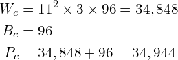
$\begin{align*}W_c &= 11^2 \times 3 \times 96 = 34,848 \\B_c &= 96 \\P_c &= 34,848 + 96 = 34,944\end{align*}$

Readers can verify the number of parameters for Conv-2, Conv-3, Conv-4, Conv-5 are 614656 , 885120, 1327488 and 884992 respectively. The total number of parameters for the Conv Layers is therefore 3,747,200. Think this is a large number? Well, wait until we see the fully connected layers. One of the benefits of the Conv Layers is that weights are shared and therefore we have fewer parameters than we would have in case of a fully connected layer.

Number of Parameters of a MaxPool Layer

There are no parameters associated with a MaxPool layer. The pool size, stride, and padding are hyperparameters.

Number of Parameters of a Fully Connected (FC) Layer

There are two kinds of fully connected layers in a CNN. The first FC layer is connected to the last Conv Layer, while later FC layers are connected to other FC layers. Let’s consider each case separately.

Case 1: Number of Parameters of a Fully Connected (FC) Layer connected to a Conv Layer

Let’s define,

$W_{cf}$ = Number of weights of a FC Layer which is connected to a Conv Layer.
$B_{cf}$ = Number of biases of a FC Layer which is connected to a Conv Layer.
$O$ = Size (width) of the output image of the previous Conv Layer.
$N$ = Number of kernels in the previous Conv Layer.
$F$ = Number of neurons in the FC Layer.

$\begin{align*}W_{cf} &= O^2 \times N \times F \\B_{cf} &= F \\P_{cf} &= W_{cf} + B_{cf}\end{align*}$

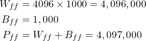
Example: The first fully connected layer of AlexNet is connected to a Conv Layer. For this layer, $O = 6$ , $N = 256$ and $F = 4096$ . Therefore,

$\begin{align*}W_{cf} &= 6^2 \times 256 \times 4096 = 37,748,736\\B_{cf} &= 4096 \\P_{cf} &= W_{cf} + B_{cf} = 37,752,832\end{align*}$

That’s an order of magnitude more than the total number of parameters of all the Conv Layers combined!

Case 2: Number of Parameters of a Fully Connected (FC) Layer connected to a FC Layer

Let’s define,

$W_{ff}$ = Number of weights of a FC Layer which is connected to an FC Layer.
$B_{ff}$ = Number of biases of a FC Layer which is connected to an FC Layer.
$P_{ff}$ = Number of parameters of a FC Layer which is connected to an FC Layer.
$F$ = Number of neurons in the FC Layer.
$F_{-1}$ = Number of neurons in the previous FC Layer.

$\begin{align*}W_{ff} &= F_{-1} \times F \\B_{ff} &= F \\P_{ff} &= W_{ff} + B_{ff}\end{align*}$

In the above equation, $F_{-1} \times F$ is the total number of connection weights from neurons of the previous FC Layer the neurons of the current FC Layer. The total number of biases is the same as the number of neurons ( $F$ ).

Example: The last fully connected layer of AlexNet is connected to an FC Layer. For this layer, $F_{-1} = 4096$ and $F = 1000$ . Therefore,

$\begin{align*}W_{ff} &= 4096 \times 1000 = 4,096,000\\B_{ff} &= 1,000 \\P_{ff} &= W_{ff} + B_{ff} = 4,097,000\end{align*}$

We leave it for the reader to verify the total number of parameters for FC-2 in AlexNet is 16,781,312.

Number of Parameters and Tensor Sizes in AlexNet

The total number of parameters in AlexNet is the sum of all parameters in the 5 Conv Layers + 3 FC Layers. It comes out to a whopping 62,378,344! The table below provides a summary.

Layer Name	Tensor Size	Weights	Biases	Parameters
Input Image	227x227x3	0	0	0
Conv-1	55x55x96	34,848	96	34,944
MaxPool-1	27x27x96	0	0	0
Conv-2	27x27x256	614,400	256	614,656
MaxPool-2	13x13x256	0	0	0
Conv-3	13x13x384	884,736	384	885,120
Conv-4	13x13x384	1,327,104	384	1,327,488
Conv-5	13x13x256	884,736	256	884,992
MaxPool-3	6x6x256	0	0	0
FC-1	4096×1	37,748,736	4,096	37,752,832
FC-2	4096×1	16,777,216	4,096	16,781,312
FC-3	1000×1	4,096,000	1,000	4,097,000
Output	1000×1	0	0	0
Total				62,378,344

Was This Article Helpful?

TRM: Tiny AI Models beating Giants on Complex Puzzles

Models with billions, or trillions, of parameters are becoming the norm. These models can write

Deploying ML on Arduino: From Blink to Think

Deploying ML on Arduino Nano 33 BLE. Explore TinyML techniques, setup steps, and why older

VideoRAG: Redefining Long-Context Video Comprehension

Discover VideoRAG, a framework that fuses graph-based reasoning and multi-modal retrieval to enhance LLMs’ ability

Was This Article Helpful?

convolutional neural network, deep learning

VideoRAG: Redefining Long-Context Video Comprehension

Discover VideoRAG, a framework that fuses graph-based reasoning and multi-modal retrieval to enhance LLMs' ability to understand multi-hour videos efficiently.

AI Agent in Action: Automating Desktop Tasks with VLMs

Agentic AIGUIVLMs

Kukil September 30, 2025

AI Agent in Action: Automating Desktop Tasks with VLMs

Learn how to build AI agent from scratch using Moondream3 and Gemini. It is a generic task based agent free from…

The Ultimate Guide To VLM Evaluation Metrics, Datasets, And Benchmarks

Computer VisionVLMs

Bhomik Sharma September 23, 2025

The Ultimate Guide To VLM Evaluation Metrics, Datasets, And Benchmarks

Get a comprehensive overview of VLM Evaluation Metrics, Benchmarks and various datasets for tasks like VQA, OCR and Image Captioning.

Subscribe to our Newsletter

Subscribe to our email newsletter to get the latest posts delivered right to your email.

Number of Parameters and Tensor Sizes in a Convolutional Neural Network (CNN)

Size of the Output Tensor (Image) of a Conv Layer

Size of Output Tensor (Image) of a MaxPool Layer

Size of the output of a Fully Connected Layer

Summary: Change in the size of the tensor through AlexNet

Number of Parameters of a Conv Layer

Number of Parameters of a MaxPool Layer

Number of Parameters of a Fully Connected (FC) Layer

Case 1: Number of Parameters of a Fully Connected (FC) Layer connected to a Conv Layer

Case 2: Number of Parameters of a Fully Connected (FC) Layer connected to a FC Layer

Number of Parameters and Tensor Sizes in AlexNet

TRM: Tiny AI Models beating Giants on Complex Puzzles

Deploying ML on Arduino: From Blink to Think

Table of Contents

Read Next

VideoRAG: Redefining Long-Context Video Comprehension

AI Agent in Action: Automating Desktop Tasks with VLMs

The Ultimate Guide To VLM Evaluation Metrics, Datasets, And Benchmarks

Subscribe to our Newsletter

Subscribe to receive the download link, receive updates, and be notified of bug fixes

Which email should I send you the download link?

Get Started with OpenCV

Number of Parameters and Tensor Sizes in a Convolutional Neural Network (CNN)

Size of the Output Tensor (Image) of a Conv Layer

Size of Output Tensor (Image) of a MaxPool Layer

Size of the output of a Fully Connected Layer

Summary: Change in the size of the tensor through AlexNet

Number of Parameters of a Conv Layer

Number of Parameters of a MaxPool Layer

Number of Parameters of a Fully Connected (FC) Layer

Case 1: Number of Parameters of a Fully Connected (FC) Layer connected to a Conv Layer

Case 2: Number of Parameters of a Fully Connected (FC) Layer connected to a FC Layer

Number of Parameters and Tensor Sizes in AlexNet

Subscribe & Download Code

TRM: Tiny AI Models beating Giants on Complex Puzzles

Deploying ML on Arduino: From Blink to Think

VideoRAG: Redefining Long-Context Video Comprehension

Table of Contents

Read Next

VideoRAG: Redefining Long-Context Video Comprehension

AI Agent in Action: Automating Desktop Tasks with VLMs

The Ultimate Guide To VLM Evaluation Metrics, Datasets, And Benchmarks

Subscribe to our Newsletter

Subscribe to receive the download link, receive updates, and be notified of bug fixes

Which email should I send you the download link?

Get Started with OpenCV