In this post, we will learn how to select the right model using Modelplace.AI. Selecting the right model will make your application faster, help you scale it to millions of requests, and save a ton of money in cloud computing costs.
Before we go into the technical details let’s understand the problem from the point of view of a n00b.
Model Selection for n00bs
Let’s say you are a programmer who is new to AI. You want to use a person detector for your camera application for a client. Now, you are not an expert in AI, but a bit of googling informs you about the numerous options you have.
The most popular among them is probably YOLO which stands for You Only Look Once. The name is ironic because you actually do not look just once!
You look at YOLO v1, v2, v3, v4, v5, v6 – ok, we got a bit carried away. There is no v6 yet, but boy there are so many options! Which one do you pick?
Confused, you take a chance on YOLO v4.
You spend your blood, sweat, and tears for the next 4 hours checking out the GitHub repo, compiling with necessary prerequisites, downloading the model, and making everything work on a Raspberry Pi only to find the model is slow.
There was a Tiny version of YOLO you missed!
So, you do this all over again for Tiny YOLO v4. It works great, and you are happy.
Your happiness evaporates when a senior AI programmer on your team asks you the reason for choosing Tiny YOLO v4 instead of Tiny YOLO v3.
You have no answer.
You had assumed that Tiny YOLO v4 would be better than Tiny YOLO v3 because you know v4 > v3.
Later, you would discover Modelplace.AI which will help you solve this problem in seconds but right now events are about to take a bad turn.
You demo your application to your client and they are not happy with the accuracy. They are ready to add more processing power to the application.
Very well, you suggest YOLO v4.
The client, whose Googling skills are superior to yours, asks you about NAS-FPN?
You have never heard about it. It is embarrassing.
To add insult to injury, they ask you about CenterNet. Yet again, you have no clue.
To save face you tell the client that you will do your research and get back to them. Now, you face the grim prospect of installing these models, finding the accuracy of every model, understanding how fast each model is, and checking its memory footprint.
AI was supposed to be fun!
In your moment of despair, you run to the one Uber AI wizard who seems to know everything. No matter what your job, there is always one such person.
She tells you about the Benchmarking tool on Modelplace.AI that changes your life forever.
Now, let’s get a bit technical.
What is Modelplace.AI?
Modelplace.AI is a large collection of AI models you can try on your own images and videos before downloading models or installing any code. In addition to qualitatively evaluating models, you can also quantitively compare models available for the same task.
Once you like the model you have a few options to use it in your application
- Web API : You can use any model or a collection of them by calling the web api.
- Python wheel : If you would rather download the model and run locally, many models are available as a downloadable python wheel which you can install using pip.
- Device specific : The website also has many models that work directly on OpenCV AI Kit. You can purchase an OAK at the OpenCV store.
Modelplace.AI is also a marketplace where developers of AI models can monetize their models. This feature is currently in beta, and you can learn more by emailing modelplace@opencv.ai.
The video below is a brief introduction to Modelplace.AI.
Benchmarking on Modelplace.AI
Comparing two models for a particular task is not as straightforward as it may seem at the outset. For example, one model may be very accurate but it may be computationally very expensive.
That is why we compare models on three different metrics and visualize them on a bubble chart on Modelplace.AI.
- Performance : A measure of inference speed. Shown long the X-axis.
- Quality : A measure of model accuracy. Shown along the Y-axis.
- Model size: A measure of model size during inference. Shown using the size of the circle.
Each chart is grouped by the task type and the dataset on which the values were obtained. For example, we compare object detection models on COCO.
How to read the benchmark
The Benchmark section is located at the bottom of the model pages.
Let’s consider Tiny YOLO v4 as an example.
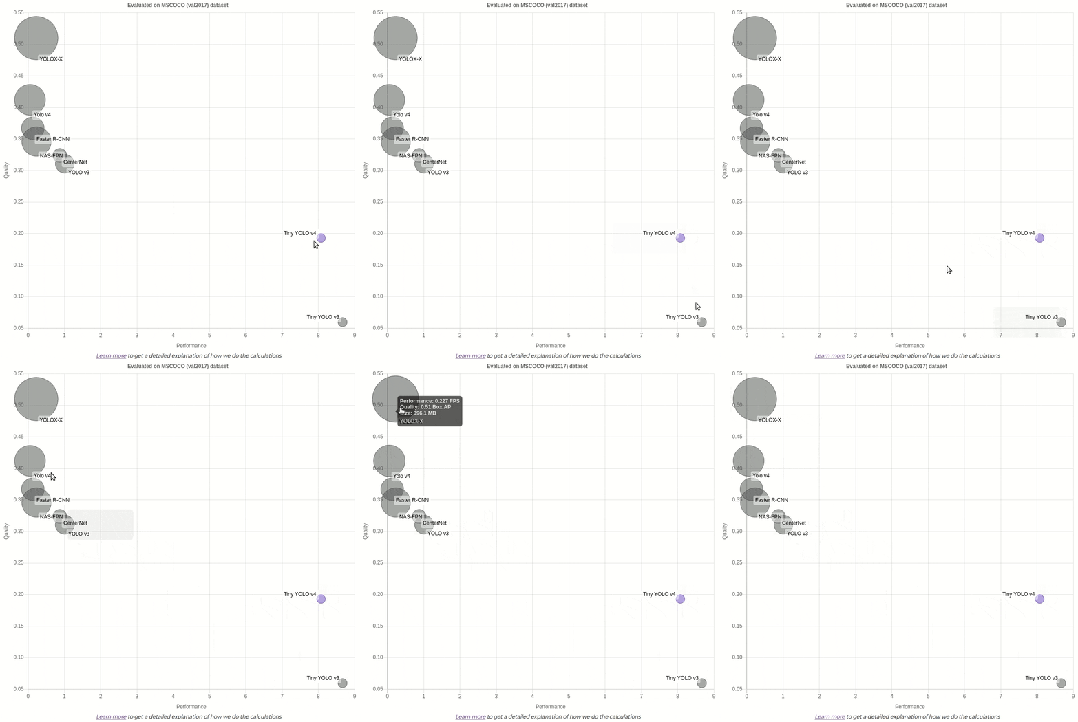
You can see that the bubble chart represents all the models with the same task type (detection) and the same validation dataset MSCOCO (val2017) as the model you are on (Tiny YOLO v4). The dataset used for evaluating the models is shown at the top of the chart. The model you are currently looking at is highlighted using a purple circle.
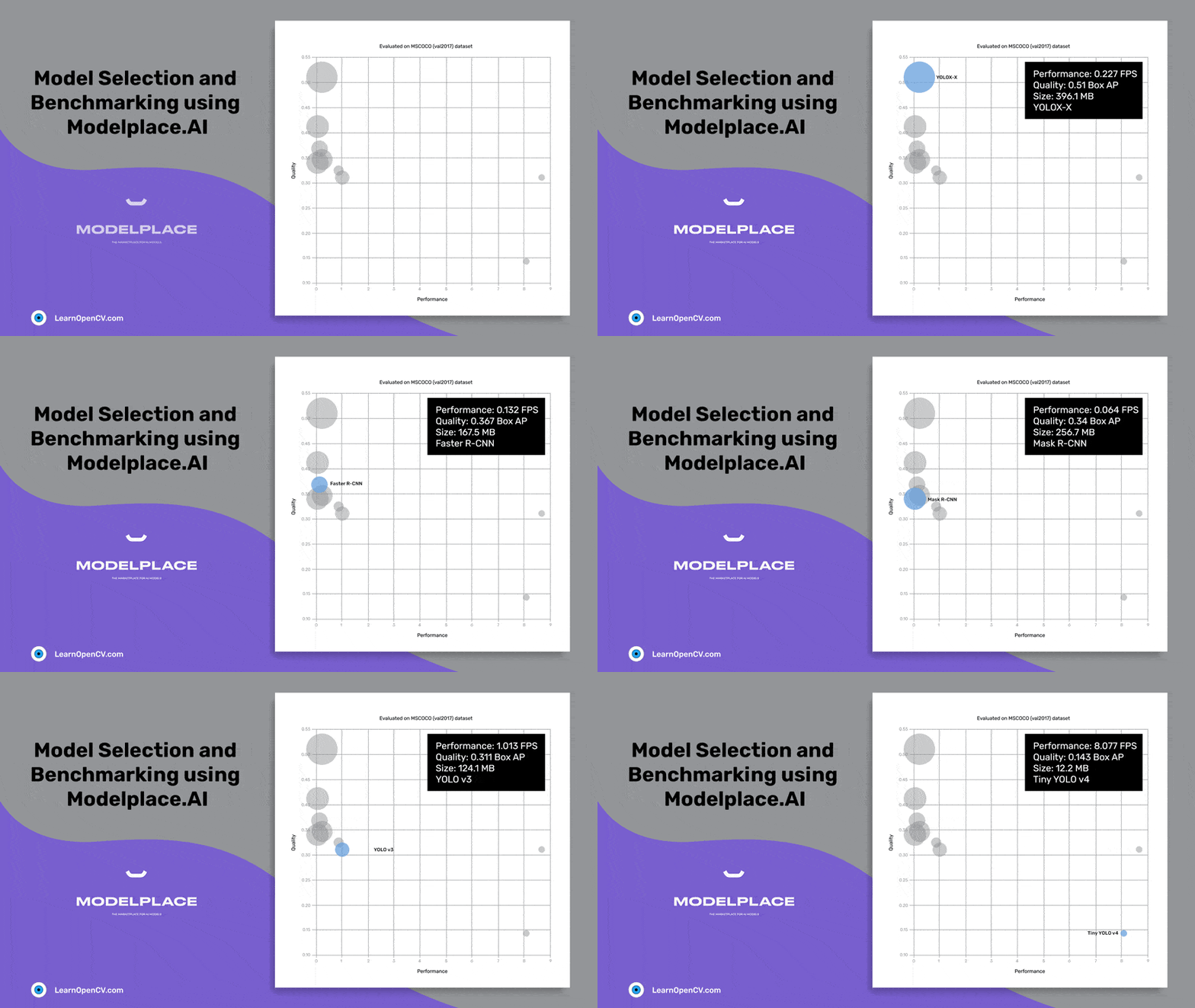
To see the specific values, you can hover your cursor over a circle.
YOLOX-X shows the best quality while Tiny YOLO v3 is way faster than the others. It also has a small memory footprint, but if you want a more accurate model without a dramatic speed decrease – Tiny YOLO v4 could be a better option.
Datasets
When possible we measure general-purpose models on public datasets such as MSCOCO or PASCAL VOC. However, for some models (e.g. the leaf detection model), we can’t measure the quality metrics as there are no large public datasets to measure their quality. Because of that, we use the value provided by the authors.
To keep it standard for all the models, we follow the two rules:
- If a model is general-purpose, it’s measured on a public dataset
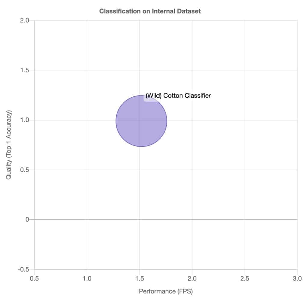
- If a model is specific, only the performance metrics are measured, while the quality value is taken from the source publication. For those models we use the Internal dataset, and if it is shown on the bubble chart.
1. Object Detection — MSCOCO (val2017).
Exceptions:
All subsets described below were obtained by using the COCO python API. By passing catIds (category indexes to be extracted from MSCOCO val2017) argument to getAnnIds function, the annotations for exact classes were extracted.
- MSCOCO (val2017 person only subset) dataset — for validation of the person/pedestrian detection models: CenterNet, Person Detector, Pedestrian Detector Adas;
- MSCOCO (val2017 vehicle only subset) dataset — for validation of the vehicle detection models: Vehicle Detector Adas;
- MSCOCO (val2017 person, vehicle and bike only subset) dataset — for validation of the PVB (person, vehicle, bike) detection models: Person Vehicle Bike Detector.
2. Landmark Detection: Wider Facial Landmarks in-the-wild dataset — for validation of the facial landmarks models: DBFace, Landmarks Regression Retail, Facial Landmarks Regression Adas.
3. Pose Estimation: MSCOCO (val2017 person keypoints subset) dataset — for validation of the pose estimation models.
4. Classification: ImageNet dataset — for validation of the classification models.
Exceptions:
- EfficientNetB4 based Cotton Vs Velvet Leaf classification from Eden Library
This model is trained on specific data so can’t be measured on a general-purpose dataset.
5. Segmentation: Pascal VOC 2012 Dataset— for validation of the segmentation models.
Exceptions:
- Supervisely Person Segmentation Dataset — for validation of DeepLabV3+;
- Cityscapes — for validation of PointRend.
6. Text Detection: CTW1500— for validation of the text detection models.
7. Emotion Recognition: AffectNet — for validation of the emotion recognition models.
Quality
We use specific metrics for measuring the quality, depending on the task type. This section provides an overview of the metrics used for each type.
1. Detection: Mean Average Precision (mAP) — mAP with several Intersection over Union (IoU) thresholds. As a final metric, we average mAP over IoU thresholds (from 0.5 to 0.95 with 0.05 step).
2. Pose Estimation: Mean Average Precision (mAP) — with Object Keypoint Similarity.
Exceptions:
Normalized Mean Absolute Error (NMAE) for Hand Landmarks Regression.
3. Landmark Detection — Normed Mean Error computed as the distance between the ground-truth and estimated landmark positions normalized by the distance. It is calculated differently depending on a model:
- For Facial Landmarks Regression and Landmarks Regression Retail, the distance between eyes we use as normalization;
- For Iris Landmark Detection, the normalization is done by using white-to-white diameter (WWD). WWD is calculated as the 3D distance between the left and right landmarks on iris contour taken from the ground truth.
4. Classification — Accuracy metric with “top-1” and “top-5” error rates.
5. Segmentation — we use Pixel Accuracy.
6. Text Detection— Precision/Recall and their modified versions TIoU-precision/TIoU-recall.
7. Tracking— MOTA. MOTA accounts for all object configuration errors made by the tracker, false positives, misses, mismatches over all frames.
Performance
The metric provided for performance measurement is FPS and calculated by the formula:
FPS = 1 / (Mean Preprocess Time + Mean Forward Time + Mean Postprocess Time)
- Mean Preprocess Time — the average time of pre-processing function execution on a batch;
- Mean Forward Time — the average time of forwarding function execution on a batch;
- Mean Postprocess Time — the average work time of post-processing function execution on a batch.
All models are evaluated with a batch size of 1.
Model Size
For size of the model we use the size of the model on disk which is a reasonable proxy for size of the model in memory.
Compute machines
All models from the same domain are inferred on the cloud machines with equal characteristics to compare them in a fairway. They are evaluated on the n1-standard-1 Google Cloud virtual machine. This machine has 1 vCPU and 3.75 GB of RAM.
Note:
We evaluate all models on vCPU, which is why the performance results are expectedly low. Please take into account the fact that with more powerful CPU performance results would be higher.
Also for comparison purposes and better performance results understanding, as an example, we evaluated CenterNet on the non-cloud machine with the following characteristics:
- Intel Core i7-8700
- 12 CPU
- 64 GB system memory
- batch size = 1
| Metric | Non-Cloud Machine | Cloud Machine |
| FPS | 4.75 | 0.87 |
| Mean Preprocess Time(seconds) | 0.0004 | 0.001 |
| Mean Postprocess Time(seconds) | 0.0005 | 0.0009 |
| Mean Forward Time(seconds) | 0.2 | 1.14 |
Troubleshooting
If anything in this document is not covered or you have any questions, please contact us at modelplace@opencv.ai.







100K+ Learners
Join Free OpenCV Bootcamp3 Hours of Learning