Modern image generation and use have exploded across the web, gaming, XR, cloud vision, and generative AI, creating an urgent need for more innovative, more adaptive visual encoding strategies. Image-GS enters this landscape as a fresh, highly efficient approach to representing images using adaptive 2D Gaussian splats, offering capabilities far beyond traditional codecs or neural implicit representations.

For decades, traditional codecs like JPEG, PNG, and more recently AVIF/WEBP have dominated the landscape. Neural implicit representations – SIREN, I-NGP, ReLU-LF – attempted to modernize image encoding by encoding images into MLPs or multi-resolution grids. But both worlds struggle to represent, transmit, and store images efficiently without losing critical detail or semantics.
Image-GS, redefining how images can be represented – not as pixels or neural fields, but as explicit, adaptive sets of colored 2D Gaussians, optimized progressively through differentiable rendering. The result is a representation paradigm that is compact, flexible, high-fidelity, hardware-friendly, content-adaptive, real-time-ready, and, most importantly, semantic-aware.
Let’s dive into the whole system.
- Why Gaussian-Based Image Representation?
- Fundamentals: Representing Images as 2D Gaussians
- The Complete Image-GS Pipeline
- Implementing the Image-GS Pipeline in Practice
- Image-GS Experimental Results
- Conclusion
- References
1. Why Gaussian-Based Image Representation?
To understand why Image-GS uses 2D Gaussians instead of pixels or neural networks, we need to step back and look at how images are traditionally represented – and why those methods break down in today’s world of high-resolution, stylized, AI-generated content.
Let’s break it down clearly.
1.1 The Limits of Pixel-Based Codecs (JPEG, PNG, WebP, AVIF)
Traditional image formats operate entirely on fixed pixel grids. This leads to several fundamental problems:
- They treat every region the same way – A flat blue sky gets the same “attention” as a detailed face or complex texture. Smooth areas get too many bits. Complex areas get too few bits. Compression becomes unbalanced.
- They introduce artifacts: at low bitrates, JPEG creates blockiness, ringing, and halos; AVIF/WebP struggle with stylized brushstrokes; and PNG stays lossless but produces huge file sizes.
These formats were designed for photography, not AI-generated art, not stylized anime, not dense textures, and especially not the non-uniform detail seen in modern images.
1.2 The Limits of Neural Implicit Image Representations
Neural implicit models encode an image as:
- a coordinate → pixel-value function
- usually implemented with an MLP or multi-resolution grid
They sound modern, but they have severe limitations:
- They require heavy computation – To decode a single pixel, the model must run through multiple neural layers, evaluate non-linear functions, and use large learned weight matrices. This makes them slow to decode, complex to deploy on GPUs, unsuitable for real-time rendering, and power-hungry on edge devices or browsers.
- They are not content-adaptive – The model’s capacity is fixed at training time – same model for a smooth background and then the same model for a highly textured area. This forces a single network to “fit everything,” which leads to blurred difficult regions, overfitting simple regions, and poor performance at low bitrates.

- They misbehave with stylized images: Neural models produce ghosting, ringing, and strange color shifts, and often fail to capture sharp, discontinuous strokes.
1.3 The Breakthrough Idea: Use 2D Gaussians
A 2D Gaussian is a smooth, elliptical “blob” with:
- a center
- a shape (covariance)
- a rotation
- a color
And significantly, Gaussians can overlap, blend, move, resize, and increase in number. They naturally represent smooth gradients and sharp edges, and they can even be optimized to match image structure.
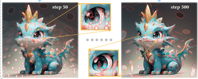
Gaussians provide natural adaptivity: few large Gaussians for smooth regions, and many small Gaussians for detailed or high-frequency regions. This is something pixels and neural fields can’t do.
2. Fundamentals: Representing Images as 2D Gaussians
To understand Image-GS, we must first understand what it means to model an image using 2D Gaussians. Let’s build the understanding step by step.
2D Gaussian
Let’s forget math for a moment, and imagine placing small, soft, colored “blobs” on a blank canvas.
Each blob:
- has a center point (where it sits)
- has a shape (circular or stretched)
- has a direction (rotation)
- has a color
- smoothly fades out toward its edges
This soft “blob” is precisely what a 2D Gaussian looks like.
Now imagine overlapping hundreds or thousands of these blobs – if placed correctly, they can reconstruct an entire image. That’s the big idea behind Image-GS.
How Image-GS Defines a Gaussian?
Each Gaussian has the following parameters:
| Parameter | Meaning | Intuition |
|---|---|---|
| μ = (x, y) | center | where the blob is placed |
| s₁, s₂ | scale | how wide or tall the blob is |
| θ | rotation | direction or tilt of the ellipse |
| c | color | the RGB (or multi-channel) value |
| Σ | covariance | mathematical form of size+shape |
Therefore, in plain English: A 2D Gaussian is a small, colored, rotated ellipse.
Image-GS uses Anisotropic Gaussians, where its spread and orientation are direction-dependent. This is in contrast to an isotropic Gaussian, which is perfectly circular or spherical and has the same properties in all directions. Technically, Anisotropic Gaussians mean:
- s₁ and s₂ can be different.
- The blob can be stretched horizontally or vertically.
- It can be rotated.
This is how they capture textures and edges very well.
How Gaussians Reconstruct an Image?
Imagine layering many transparent, soft ellipses on top of each other. Each pixel in the final image is produced by:
Combining contributions from the Gaussians that overlap that pixel.
Mathematically, it’s just a weighted average. Intuitively, it’s like – “If many blobs contribute to this pixel, mix their colors based on how strongly they cover that area.”
So:
- A Gaussian covering a pixel firmly → gives more color influence
- A Gaussian far away → gives almost no influence
This creates smooth, natural-looking reconstructions. We will be discussing the entire pipeline in great detail in this blog post.
The Key Superpower: Content-Adaptivity
A Gaussian can stretch or compress to fit content.
Image-GS starts with a coarse set of Gaussians and progressively refines by:
- Adding more Gaussians in areas with great detail
- Leaving smooth regions with fewer, bigger Gaussians
- Adjusting shapes to match actual edges and textures
Examples:
- Large Gaussian → flat sky
- Tall Gaussian → vertical building edge
- Thin horizontal Gaussian → hair strand
- Rotated Gaussian → brush stroke direction
This is precisely what classic codecs and neural fields cannot do.
3. The Complete Image-GS Pipeline
The Image-GS framework transforms a standard image into a compact, content-adaptive, Gaussian-based representation through a multi-stage pipeline. Unlike traditional codecs or neural implicit models, Image-GS builds a continuous image representation using thousands of optimizable 2D Gaussians.
Below is the complete flow – from raw input all the way to final, upsampled output.
3.1 Input Image Preprocessing
The pipeline begins with loading the raw input image:
- A 2D RGB image of size H×W
- Pixel values normalized to [0,1]
- Converted into a tensor suitable for PyTorch
Let the input image be:
![]() → [0,1]
→ [0,1]
3.2 Gradient Magnitude Map
An image gradient measures how rapidly the pixel colors change in a given direction. Image-GS computes the image gradient magnitude, which reveals edges and high-frequency regions. For each pixel x, Image-GS evaluates horizontal and vertical changes. Using Sobel filters or a high-pass convolution:

This gradient map highlights:
- strong edges
- structure
- contours
- texture regions
For each pixel x, Image-GS evaluates horizontal and vertical changes:
- Bright lines = strong edges / important structure
- Dark regions = smooth / low-detail regions
This map is later used to decide where to place more Gaussians during initialization.
3.3 Content-Adaptive Gaussian Initialization
Instead of placing Gaussians uniformly, Image-GS allocates them based on content importance. It uses the gradient map to compute a sampling probability:

Where:
- First term → edge strength. This term ensures – high-gradient pixels → high probability, and low-gradient pixels → low probability. It means edges, corners, curves, textures, etc., receive more initial Gaussians.
- Second term → uniform fallback. This term ensures that every pixel gets at least some chance, that flat regions are not ignored, and that the representation doesn’t leave “holes”.
 ≈ 0.1
≈ 0.1
Intuition
- Edgy, detailed areas → high probability → more Gaussians
- Smooth areas → low probability → fewer Gaussians
3.4 Representing Pixels using 2D Gaussians
Once Image-GS has placed its initial Gaussians, the next question is: How do these Gaussians actually reconstruct the image?
First of all, a 2D Gaussian has the form:

Where the covariance matrix is:
![]()
that directly controls how wide the Gaussian spreads, whether it is circular or elongated, its rotation angle, and its anisotropy (different spreads in different directions), with the help of:
- rotation matrix R
- scale matrix
 , in which changing
  → widen/narrow horizontally, changing
  → widen/narrow vertically, and changing
  → rotate the ellipse.
This parameterization supports anisotropic (stretched/rotated) splats, giving Image-GS excellent edge and texture representation. Before moving on to the next pipeline step, let’s recall that in Image-GS, color is not view-dependent (unlike 3D Gaussian Splatting); instead, each 2D Gaussian stores a color vector.
3.5 Differentiable Gaussian Rendering in Image-GS
To render the image from Gaussians, each pixel color is computed as a weighted blend of nearby Gaussians:

Intuition:
- If a Gaussian strongly overlaps a pixel, it contributes more color
- If it’s far away, it contributes almost nothing
- Multiple Gaussians combine smoothly to form the final color
This eliminates blocking artifacts, aliasing, jagged edges, and hard transitions.
But evaluating all Gaussians per pixel is too expensive. Therefore, Image-GS uses:
Tile-Based Rendering
- The image is divided into tiles.
- Only Gaussians whose ellipses intersect each tile are considered.
Top-K Gaussian Pruning
For each pixel x, Image-GS keeps only the K strongest Gaussians:
![]()
Final rendering:

This top-K pruning improves both:
- computational efficiency
- reconstruction quality (as shown by ablation studies)
3.6 Optimization via Gradient Descent
The reconstruction is optimized by minimizing:

This encourages:
- pixel-level accuracy, which is accountable for measuring the absolute difference between reconstructed and original pixels, ensuring correct colors, and then ensuring low per-pixel error, too
- structural integrity loss encourages the reconstruction to “look” correct to the human eye
- smoother edges
- better perceptual quality
Trained Parameters
During optimization, the following are updated:
- Gaussian positions μi, which move Gaussians in the image
- Scales
 , which shrinks or stretches the ellipse
 - Rotations
 , which rotates the ellipse to match the edges
 - Colors
 , which changes the Gaussian’s color
This process makes Gaussians “snap” into place, aligning with edges, strokes, textures, and color regions. Technically, through this process, Gaussians shift into the right places, scales shrink or grow, rotations align with the edges, and colors become more accurate.
3.7 Progressive Gaussian Addition (Content-Aware Refinement)
Image-GS adds more Gaussians where reconstruction error is high. Sampling probability for new Gaussians:

This ensures:
- Complex regions get more Gaussians.
- Simple regions get fewer Gaussians.
- Gaussian budget is used efficiently.
- PSNR/SSIM improves over training
This matches the log outputs we will see later on when implementing the Image-GS pipeline.

3.8 Final Reconstruction
The final optimized set of Gaussians produces:
- high PSNR (Peak Signal-to-Noise Ratio PSNR measures pixel-level accuracy between the reconstructed image and the ground truth) values (≈ 40 dB)
- high SSIM (Structural Similarity Index SSIM evaluates structural similarity between two images by considering luminance, contrast, texture, spatial structure, and local patterns) values (≈ 0.97–0.98)
- visually crisp images with low distortion
- excellent performance on stylized images
The output image looks nearly identical to the input – often smoother and cleaner due to Gaussian blending.
Upsampled Reconstruction (Super-Resolution for Free)
A key advantage of Image-GS is that Gaussians are continuous functions rather than discrete pixels. So Image-GS can render the image at various scales, without pixelation.
![]() is defined for any x ∈
is defined for any x ∈ ![]()
Thus, rendering at higher resolutions simply means evaluating Gaussians at more locations.
4. Implementing the Image-GS Pipeline in Practice
A Quick Note on Linux (Why We Switched to Windows)
Our original plan was to run Image-GS on a Linux-based system using the official environment.yml and README instructions. In theory, it was straightforward; in practice, we repeatedly ran into C++/CUDA extension + PyTorch ABI issues.
Two main problems kept showing up:
fused-ssimbuild failure – Installingfused-ssim(as recommended in the README) caused this error:
ImportError: .../torch/lib/libtorch_cpu.so: undefined symbol: iJIT_NotifyEvent
This is due to an ABI mismatch between the compiled PyTorch library and the C++ extension. Modern PyTorch wheels no longer expose that symbol. The critical realization: Image-GS no longer needs fused-ssim; it uses pytorch-msssim instead. So this step is safe to skip.
gsplatextension failure with the same symbol error
Building gsplat on Linux hit the same iJIT_NotifyEvent issue, this time from gsplat’s CUDA extension linking against PyTorch. Fixing this requires a very careful combination of conda-only PyTorch builds, matching CUDA versions, and avoiding interference from system Intel/oneAPI libraries. It’s doable, but not worth the friction if you just want to experiment with Image-GS.
Because of repeated ABI headaches on Linux, we chose a more practical approach for this blog: use Windows for the hands-on pipeline, which turned out to be much smoother once we pinned the right versions and flags.
Image-GS Implementation on Windows: Step-by-Step
- First, clone the Image-GS Repository by running the following command in Shell:
git clone https://github.com/NYU-ICL/image-gs.git
cd image-gs
- Create the conda environment from
environment.yml
conda env create -f environment.yml
conda activate image-gs
- Include
fused-ssim
pip install git+https://github.com/rahul-goel/fused-ssim/ --no-build-isolation
- Install
gsplat(Correct Version, Correct Build Flags). Two things matter here:- We must avoid pip’s “build isolation” (or the build won’t see torch).
- We must use a compatible gsplat version (1.3.x), because 1.4.0 changed the API.
--no-build-isolation→ prevents pip from creating a temporary, torch-less build environment.--no-deps→ avoids pip trying to “helpfully” reinstall a different torch.
cd gsplat

# Make sure we use this env's Python
pip install --upgrade pip setuptools wheel

# Install a compatible gsplat version
pip install gsplat==1.3.0 --no-build-isolation --no-deps
- Install the Image-GS Package Itself while still using the same torch & gsplat we’ve already set up.
cd ..
python -m pip install -e . --no-build-isolation --no-deps
- The Python script (model.py) has to be replaced with the original model.py Python script, which was cloned into the system while cloning the Image-GS repository. Because of some updates to the file structure, a few imports are wrong, along with some script names, which is why the replacement of the model.py Python script is necessary. The concerned Python script, along with all the instructions, can be downloaded by clicking the Download Code button, right before the “Implementing the Image-GS Pipeline in Practice” section of the blog post.
Once everything is installed, running Image-GS on an example image is straightforward.
5. Image-GS Experimental Results
Download the image and texture datasets from OneDrive and organize the folder structure as follows –
image-gs
└── media
    ├── images
    └── textures
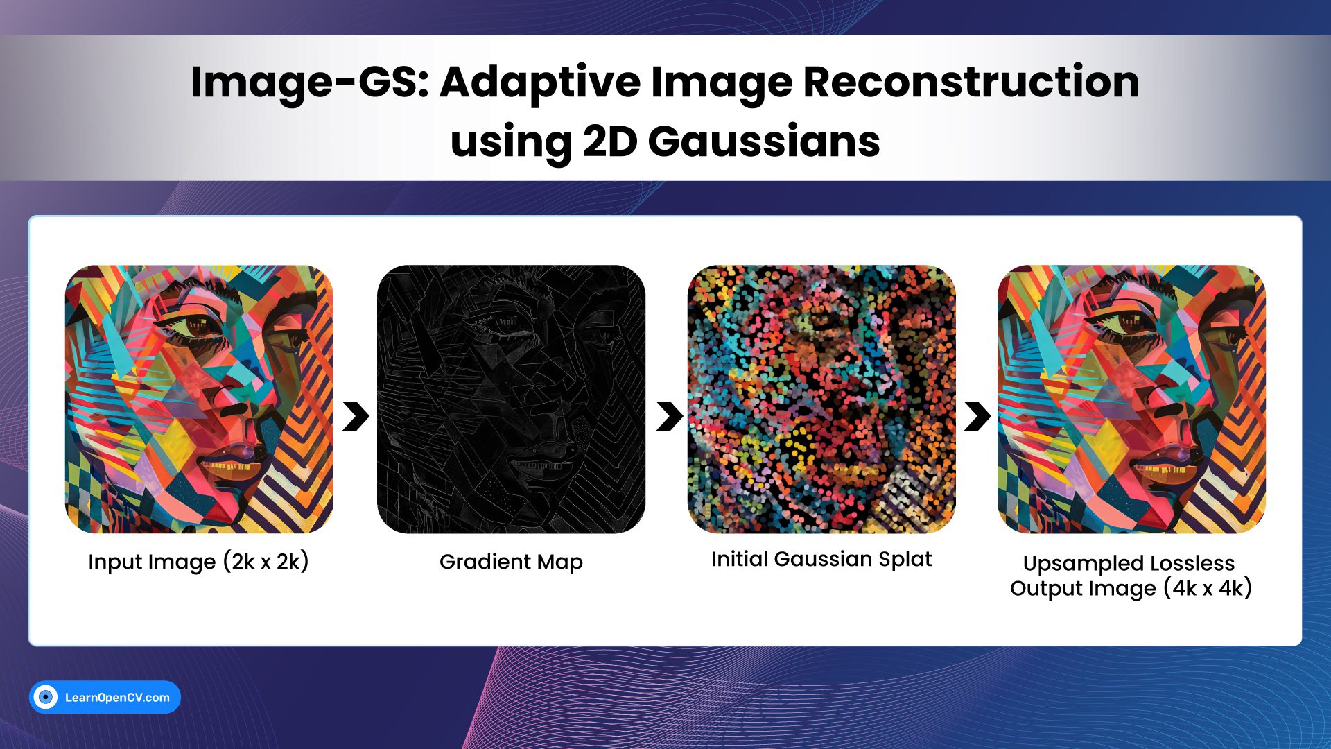
To appreciate how Image-GS reconstructs images using adaptive 2D Gaussians, it helps to visualize the intermediate outputs produced during the optimization pipeline. Here, we walk through four key results generated from a sample input image, explaining what each output represents and how it fits into the overall pipeline.
These images together reveal the entire story: how Image-GS analyzes the input, initializes Gaussians, refines them, and ultimately produces a smooth, high-fidelity reconstruction capable of upsampling far beyond the original resolution.
Input Image (2k x 2k size)

Shell command to reconstruct the input image
python main.py --input_path="images/art-5_2k.png" --exp_name="test/art-5_2k" --num_gaussians=10000 --quantize
Reconstructed Outputs
Shell Logs –

Gradient Magnitude Map Output –
The first output is the gradient magnitude map, a visualization of the image’s high-frequency information, such as edges, curves, and fine details.
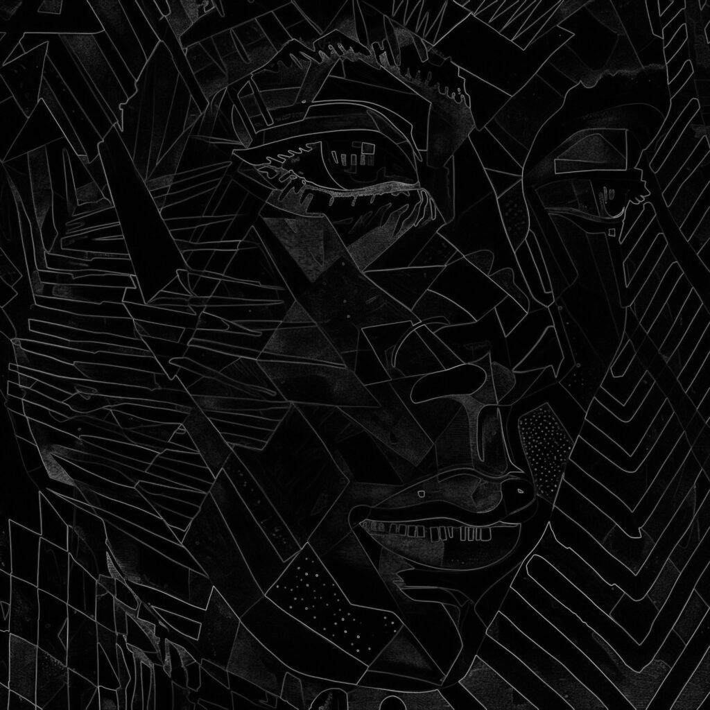
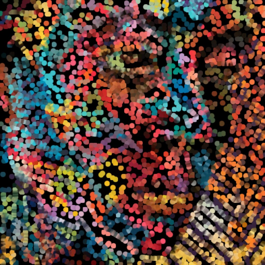
Initial Gaussian Splat (Step 0) Output – The second output represents the initial Gaussian distribution, before any optimization has taken place. At this stage, Gaussians are placed using the content-adaptive sampling strategy, colors come directly from sampled pixels, shapes and rotations are still coarse, the reconstruction is rough and blurry, and PSNR and SSIM are very low (as expected)
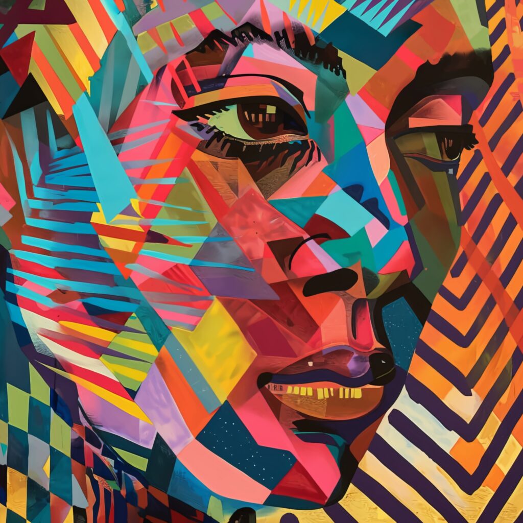
Final Output (Reconstructed Image) – The third output is the final optimized reconstruction, produced after thousands of gradient descent steps and several rounds of Gaussian refinement.
Shell command to render the upsampled image with size 4k x 4k –
python main.py --input_path="images/art-5_2k.png" --exp_name="test/art-5_2k" --num_gaussians=10000 --quantize --eval --render_height=4000
Shell Logs –
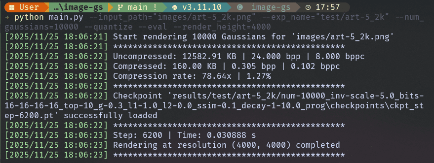
Upsampled Lossless Output –

Limitations of Image-GS
Image-GS is powerful but not perfect.
- Hard to batch-process – Each image uses a different number of Gaussians → not batch-friendly.
- Training is content-adaptive – Makes it slightly unpredictable for standardized pipelines.
- Not yet optimized for video – But planned.
6. Conclusion
Image-GS is more than an image compression technique. It is a fundamental reformulation of image representation, leveraging adaptive 2D Gaussian primitives to achieve a unique blend of:
- fidelity
- efficiency
- semantic retention
- smooth level-of-detail
- restoration properties
- GPU-friendly execution
- texture compatibility
Its explicit, differentiable, content-aware design allows it to outperform classical and neural codecs alike – especially on AI-generated, stylized, and multispectral content. As Gaussian methods continue to reshape computer vision and graphics, Image-GS stands as a major step toward the future of universal, adaptive, and intelligent visual representations.







100K+ Learners
Join Free OpenCV Bootcamp3 Hours of Learning