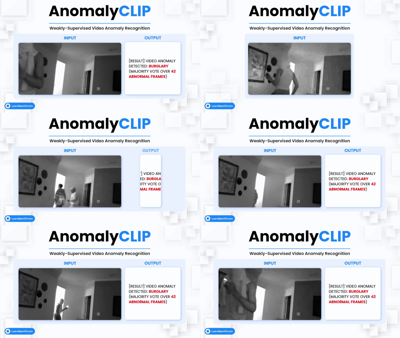
Video Anomaly Detection (VAD) is one of the most challenging problems in computer vision. It involves identifying rare, abnormal events in videos – such as burglary, fighting, or accidents – amidst overwhelmingly normal footage. Traditional methods either rely on expensive frame-level annotations, unsupervised heuristics, or one-class classification using only normal data.
But VAD alone is no longer enough. Beyond simply detecting that something unusual is happening, there is a growing need for Video Anomaly Recognition (VAR) – classifying what anomaly occurred. For example, distinguishing between a “Robbery” and an “Arson” provides actionable insights for surveillance and monitoring systems.
This is where AnomalyCLIP comes in. It is a new framework that extends CLIP’s powerful vision-language representations to the anomaly detection domain, allowing models to both detect and recognize anomalous events under weak supervision.
- Why AnomalyCLIP?
- The AnomalyCLIP Framework
- Implementing AnomalyCLIP for Video Anomaly Recognition
- Ablation Studies: Why AnomalyCLIP Works
- Key Takeaways
- Conclusion
- References
1. Why AnomalyCLIP?
Video anomaly detection has been studied for years, but existing approaches have critical shortcomings. To understand why AnomalyCLIP is needed, let’s break this down.
1.1 Traditional Approaches and Their Limits
One-Class Classification
- Train only on normal videos.
- At test time, any deviation from normal is flagged as an anomaly.
- Limitation: struggles with “uncommon but normal” behaviors (e.g., someone running to catch a bus looks like an anomaly).
Unsupervised Methods
- Require no labels.
- Often reconstruction- or prediction-based (e.g., predict next frame and compare).
- Limitation: weak discriminative power in complex, real-world settings.
Fully-Supervised Methods
- Train with frame-level annotations.
- Performs well, but annotation cost is prohibitive – imagine labeling 200k frames manually.
Weakly-Supervised Methods (current trend)
- Use only video-level labels (normal/anomalous).
- Popularized by Sultani et al. (2018) with an MIL (Multiple Instance Learning) framework.
- Later methods (RTFM, S3R, SSRL) improved segment selection and temporal modeling.
- Limitation: still mainly binary (normal vs anomaly), unable to recognize anomaly type.
1.2 Why Recognition Matters (VAR vs VAD)
- VAD (Detection): answers “Is there an anomaly in this video?”
- VAR (Recognition): goes further – “What anomaly occurred? Was it Burglary? Fighting? Explosion?”
This shift is critical for practical use cases:
- Surveillance: Different responses for “Burglary” vs “Explosion”.
- Healthcare monitoring: Distinguish “Fall” vs “Seizure”.
- Traffic systems: Separate “Accident” vs “Vandalism”.
Yet, no existing weakly-supervised method addressed VAR effectively – until AnomalyCLIP.
1.3 Opportunity with CLIP
- CLIP (Radford et al., 2021) aligns images with natural language descriptions.
- Learns a joint vision-language space where “a photo of a dog” is close to dog images.
- Huge potential: use text prompts to define anomaly classes (Burglary, Shooting, etc.).
- But the problem:
- Raw CLIP embeddings overlap too closely for fine-grained anomaly detection.
- Magnitudes don’t map to anomaly severity.
- Zero-shot CLIP struggles to separate normal vs anomaly.
1.4 How AnomalyCLIP Is Different
AnomalyCLIP re-engineers CLIP’s latent space for Video Anomaly Recognition under weak supervision by:
- Re-centering features around a normality prototype:
- Now magnitude = anomaly likelihood, direction = anomaly type.
- Selector Model (Semantic MIL):
- Learns anomaly directions using CoOp prompt learning.
- Robustly picks abnormal vs normal segments.
- Temporal Model (Axial Transformer):
- Models both short-term and long-term dependencies.
- Provides consistent anomaly predictions over time.
- Multi-Loss Training Objective:
- Directional losses, normal suppression, sparsity, smoothness.
- Balances detection + classification, ensures stable learning.
1.5 The Payoff
- First LLV (Large Language Vision) approach for VAR.
- Works under weak supervision (no frame-level labels).
- Outperforms SOTA on ShanghaiTech, UCF-Crime, and XD-Violence datasets.
- Detects anomalies and recognizes their types – a step beyond binary VAD.
2. The AnomalyCLIP Framework
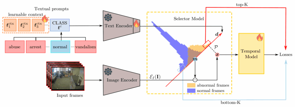
AnomalyCLIP is built upon CLIP’s vision-language alignment, but adapts and extends it specifically for weakly supervised video anomaly recognition (VAR). Its core strength lies in transforming CLIP’s latent space so that anomalies can be detected and classified using only video-level labels. Let’s break down the framework step by step.
2.1 Re-centering the CLIP Feature Space
- CLIP provides embeddings for both images and text prompts in a joint semantic space.
- However, in its raw form, CLIP cannot separate subtle anomaly classes – directions overlap, and feature magnitudes don’t reflect anomaly severity.
- AnomalyCLIP introduces a normality prototype m:
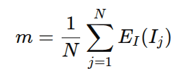
where E(I) is CLIP’s image encoder, and the sum is over all standard frames.
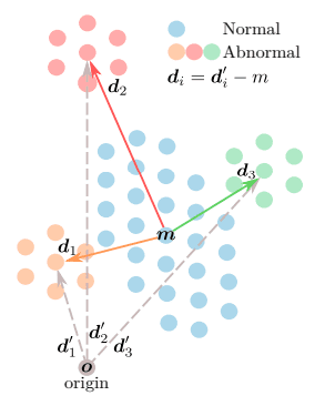
- Each frame feature is re-centered:

- Each anomaly class has its own direction vector:

where ![]() is CLIP’s text encoder,
is CLIP’s text encoder, ![]() are learnable CoOp context tokens, and
are learnable CoOp context tokens, and ![]() is the anomaly class name.
is the anomaly class name.
Interpretation:
- Magnitude of x = how abnormal the frame is.
- Direction of x = which anomaly type it belongs to.
2.2 The Selector Model (Semantic MIL)
- Real-world videos contain long stretches of normal frames, even in anomalous videos.
- AnomalyCLIP uses Multiple Instance Learning (MIL):
- Top-K frames/segments = most abnormal.
- Bottom-K frames/segments = most normal.
- Likelihood of anomaly for frame x projected onto class direction
 :
:

where BN = BatchNorm (no affine) → keeps regular features near origin, anomalies in right-tail.
- Segment-level likelihood:
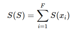
- Selector learns to discriminate anomalies vs normal in CLIP space by optimizing directional losses.
Function:
- Selects the “right” instances (frames) for training.
- Expands anomaly-normal separation.
- Provides more reliable signals for the Temporal Model.
2.3 The Temporal Model (Axial Transformer)
- The Selector alone is time-independent – it judges frames in isolation.
- But anomalies are often temporal patterns (e.g., fighting involves multiple frames).
- AnomalyCLIP uses an Axial Transformer (Ho et al., 2019):
- Applies attention along one axis at a time (segments vs frames).
- Efficient → reduces computation vs. full Transformers.
- Less prone to overfitting than Multi-Scale Temporal Networks (RTFM/SSRL).
- Captures both short-term relationships (between consecutive frames) and long-term dependencies (across distant segments).
- Outputs:
- Refined anomaly score per frame.
- Class-conditioned probabilities.
Benefit:
Adds temporal context → robust recognition of anomaly patterns.
2.4 Training AnomalyCLIP with Multiple Losses
To make Selector + Temporal work under weak supervision, AnomalyCLIP uses a combination of MIL losses and regularizers:
| Loss | Purpose |
|---|---|
| Directional anomaly loss on top-K segments | |
| Temporal anomaly classification loss | |
| Encourage bottom-K anomaly video frames to be Normal | |
| Suppress anomaly likelihoods in Normal videos | |
| Ensure top-K includes some normality | |
| Sparsity: A few frames should be abnormal | |
| Smoothness: consecutive frames are consistent |
Final Objective:

Effect:
- Selector learns reliable anomaly directions.
- The temporal model refines predictions using temporal cues.
- Regularization ensures sparse, smooth, and realistic anomaly activations.
2.5 Prediction and Aggregation
- Frame-level: anomaly scores + per-class probabilities.
- Segment-level: aggregated likelihoods from MIL.
- Video-level:
- Mean probabilities across abnormal frames.
- Top-K% frame aggregation.
- Majority vote (our implementation):
- For each abnormal frame, pick its most likely anomaly class.
- Count votes across frames.
- Dominant class = video-level anomaly label.
2.6 Why It Works
- Re-centering → aligns CLIP space with anomaly task.
- Selector model → robustly identifies abnormal snippets with MIL.
- CoOp prompts → learn anomaly-aware directions in text space.
- Axial Transformer → adds temporal reasoning.
- Loss design → balances anomaly recognition, normal suppression, sparsity, and smoothness.
Together, these innovations make AnomalyCLIP the first large language-vision model (LLV) based approach for Video Anomaly Recognition, and the first to achieve state-of-the-art performance across ShanghaiTech, UCF-Crime, and XD-Violence.
3. Implementing AnomalyCLIP for Video Anomaly Recognition
One of the most interesting aspects of working with AnomalyCLIP is that the official checkpoint does not include the complete CLIP backbone. Instead, it only stores the weights of the Selector model and the Temporal Transformer, since CLIP’s image encoder was frozen during training. This design choice impacts how we can actually run inference, and it led us to build two complementary implementation pipelines. Scripts for both of the implementations have been compiled and can be downloaded by clicking the Download Code button present a little below.
While setting up the AnomalyCLIP VAR GitHub repository, you may encounter dependency conflicts due to mismatched package versions. This is quite common with research code and can happen if your local environment has newer or older library releases than what the project expects. There are two reliable ways to fix this out of which one will definitely resolve the issue, and those ways are:
- re-install all the dependencies listed in
requirements.txtusingpip==24.0, which handles version resolution more robustly
- remove the versions of the dependencies mentioned in the
requirements.txtfile, and then run the set of commands provided below in the exact order after facing a specific error while installing the dependencies listed in therequirements.txtto manually align dependency versions and resolve conflicts.
pip install psutil
pip install imageio
pip install cloudpickle==1.2.0
pexpect==4.8
decorator
pandocfilters==1.4.1
bleach[css]==5.0.1
beautifulsoup4
Now, let’s move to the implementation part.
3.1 Using Pre-Extracted Features (.npy + Checkpoint)
In the official training setup, all videos are first processed through CLIP’s visual encoder, and the resulting features are stored in .npy files (each row corresponds to a frame/segment embedding of dimension 512).
For arbitrary videos, we rebuilt the end-to-end pipeline by adding back the CLIP encoder.
def build_net_args(labels_file, arch="ViT-B/16"):
    return dict(
        # --- from anomaly_clip_ucfcrime.yaml ---
        arch=arch,
        shared_context=False,
        ctx_init="",
        n_ctx=8,
        seg_length=16,
        num_segments=32,
        select_idx_dropout_topk=0.7,
        select_idx_dropout_bottomk=0.7,
        heads=8,
        dim_heads=None,              # OK to leave None unless our code requires a number
        concat_features=False,
        emb_size=256,
        depth=1,
        num_topk=3,
        num_bottomk=3,
        labels_file=labels_file,
        normal_id=7,                 # <-- set to your actual "Normal" id if not 0
        dropout_prob=0.0,
        temporal_module="axial",
        direction_module="learned_encoder_finetune",
        selector_module="directions",
        batch_norm=True,
        feature_size=512,
        use_similarity_as_features=False,

        # --- crucial fix ---
        ctx_dim=512,                 # <— make this an INT so PromptLearner gets 512, not a DotMap

        # --- single‑video equivalents for ${data.*} ---
        load_from_features=True,
        stride=1,
        ncrops=1,
    )
- How it works:
- Load a
.npyfile containing pre-extracted CLIP features. - Pass features into the Selector and Temporal modules using the pretrained checkpoint.
- Obtain frame-level anomaly scores and probabilities.
- Load a
def load_feats(path, normalize=False, device="cpu"):
    x = np.load(path)  # [T, D]
    if x.ndim != 2:
        raise ValueError(f"{path} must be [T, D], got {x.shape}")
    t, d = x.shape
    x = torch.tensor(x, dtype=torch.float32, device=device)
    if normalize:
        x = F.normalize(x, dim=-1)
    # AnomalyCLIP (test_mode, load_from_features=True) expects [B, NC, T, D]
    x = x.unsqueeze(0).unsqueeze(0)  # [1,1,T,D]
    return x, t, d
The above code loads a .npy file containing pre-extracted CLIP features in which each row corresponds to a frame/segment embedding of dimension 512.
# 1) Build net with the SAME args as training
net_kwargs = build_net_args(labels_file=args.labels_file, arch=args.arch)
net = AnomalyCLIP(**net_kwargs).to(device).eval()

# 2) Load only net.* weights from the checkpoint
load_net_weights_from_ckpt(net, args.ckpt, strict=False, device=device)

# 3) Features + labels + ncentroid
feats, T, D = load_feats(args.feats, normalize=args.normalize, device=device)  # [1,1,T,D]
The above code block first constructs the network (net) with the same configuration used during training. Then it loads the Selector and Temporal module weights (net.*) from the pretrained checkpoint. Finally, it prepares the input features (feats) along with their dimensions (T = number of frames, D = feature size), and sets up the normality prototype (ncentroid) for evaluation.
- Limitation:
- This only works if
.npyfiles for a video already exist, i.e., videos from the training or testing datasets (ShanghaiTech, UCF-Crime, XD-Violence). - We cannot simply pass an arbitrary raw video because the checkpoint doesn’t contain the CLIP encoder to generate features on the fly.
- This only works if
3.2 Using Raw Videos (Frames + Checkpoint)
To overcome the .npy limitation, we extended the pipeline to support any raw video file (e.g., .mp4, .avi).
- Steps:
- Sample frames from the video at a chosen FPS.
- Preprocess frames using CLIP’s normalization (resize, crop, standardize).
- Pass frames through the CLIP visual encoder (from the repo’s
anomalyclipmodule) to obtain[T,512]features. - Forward these features into the pretrained Selector and Temporal modules (loaded from the checkpoint).
- Generate frame-level anomaly scores, per-class probabilities, and video-level predictions.
def build_clip_preprocess():
    clip_mean = (0.48145466, 0.4578275, 0.40821073)
    clip_std = (0.26862954, 0.26130258, 0.27577711)
    return transforms.Compose([
        transforms.Resize(224, interpolation=transforms.InterpolationMode.BICUBIC),
        transforms.CenterCrop(224),
        transforms.ToTensor(),
        transforms.Normalize(clip_mean, clip_std),
    ])
The above code snippet preprocesses frames using CLIP’s normalization.
def compute_ncentroid_from_frames(tensor_frames, net, device, batch=64):
    feats = []
    with torch.no_grad():
        for i in range(0, tensor_frames.shape[0], batch):
            x = tensor_frames[i:i+batch].to(device)
            f = net.image_encoder(x.float())  # [B,512]
            f = F.normalize(f, dim=-1)
            feats.append(f)
    return torch.cat(feats, dim=0).mean(dim=0)
The above function computes the mean CLIP embedding across all frames of a video. That mean = ncentroid = the normality prototype (a reference point in feature space). Later, all frame embeddings are re-centered. This allows AnomalyCLIP to measure distance from normal. If close → likely normal. If far in a certain direction → abnormal, and the direction tells us which anomaly type.
- Why it works:
- Even though the checkpoint lacks CLIP encoder weights, we can still instantiate CLIP (frozen, as in training) and reuse it for feature extraction.
- By reconstructing the full AnomalyCLIP pipeline (CLIP encoders + prompt learner + Selector + Temporal), we can evaluate on any unseen video, not just the benchmark datasets.
3.3 Our Extensions
In our implementation, we went further and added:
- Frame saving: sampled frames are stored to disk for inspection.
- Per-class probabilities: CSV output includes
Normal+ anomaly classes. - Video-level prediction:
- Beyond scores per frame, we implemented a majority vote classifier across abnormal frames to decide the dominant anomaly class.
Example CSV Structure
| idx | src_frame_idx | time_sec | score | Normal | Abuse | Arrest | Burglary | … |
|---|---|---|---|---|---|---|---|---|
| 0 | 0 | 0.0 | 0.05 | 0.93 | 0.01 | 0.01 | 0.02 | … |
| 1 | 20 | 1.0 | 0.74 | 0.21 | 0.03 | 0.02 | 0.70 | … |
3.4 Inferencing Results for AnomalyCLIP on Raw Videos
Terminal command to trigger the inferencing script
python infer_raw_frames.py --video /home/opencvuniv/Work/Shubham/AnomalyCLIP/Arrest019_x264.mp4 --ckpt /home/opencvuniv/Work/Shubham/AnomalyCLIP/checkpoints/ucfcrime/last.ckpt --labels_file /home/opencvuniv/Work/Shubham/AnomalyCLIP/data/ucf_labels.csv --out outputs_single/arrest.csv --fps 8 --normal_id 7 --out_frames_dir outputs_frames
Input Video
AnomalyCLIP Output

4. Ablation Studies: Why AnomalyCLIP Works
Ablation studies are crucial for understanding which components of a model truly drive performance. In AnomalyCLIP, the authors conducted extensive experiments on UCF-Crime to validate each architectural choice, representation strategy, and loss design.
Let’s unpack the findings.
4.1 Representation & Learning of Anomaly Directions
One of AnomalyCLIP’s core innovations is learning class-specific anomaly directions in CLIP space using CoOp (Context Optimization).
- Direct optimization (no CoOp): Very poor mAUC (~70). Shows raw feature space is not aligned for anomaly recognition.
- Frozen engineered prompts (e.g., “a video from CCTV of [class]”): Better (~81 mAUC), but limited.
- Frozen CoOp: Improves further (~87 mAUC) because context tokens adapt better.
- Finetuned CoOp + unfreezing CLIP text projection (final choice): Best (~90.67 mAUC).
Takeaway:
- Learnable prompts must be tuned jointly with the CLIP text encoder for anomaly recognition.
- Random or frozen prompts fail to capture subtle differences, such as the distinction between burglary and robbery.
4.2 Number & Type of Context Vectors
How many context tokens should each class prompt have?
- Shared context (8 tokens for all classes): ~90 mAUC.
- Class-specific context (8 tokens): ~90.6 mAUC (final).
- Class-specific context (16 tokens): ~90.6 mAUC but less efficient.
Takeaway:
- Although using 4 context vectors results in a slightly higher mAUC score, the authors still chose to use 8 context vectors because they produce a higher AUC score.
- Eight tokens per class is the sweet spot: expressive enough, but not overfitting.
4.3 Likelihood Estimation & Re-centering
Three approaches were compared for anomaly likelihood:
| Method | AUC | mAUC |
|---|---|---|
| Cosine similarity (zero-shot CLIP) | 85.6 | 83.7 |
| Feature magnitude (no re-centering) | 84.9 | 89.8 |
| Re-centered features (AnomalyCLIP) | 86.4 | 90.67 |
Takeaway:
- Cosine sim → fails, confirms naïve CLIP is not VAR-ready.
- Magnitude-only → somewhat helpful but noisy.
- Re-centering transformation (subtract normal prototype) is critical – it maps anomaly degree to magnitude and type to direction.
4.4 Temporal Model Architecture
Why an Axial Transformer?
| Model | Short-term | Long-term | mAUC |
|---|---|---|---|
| MLP | ✗ | ✗ | 84.5 |
| Transformer (short only) | ✓ | ✗ | 88.4 |
| Transformer (long only) | ✗ | ✓ | 89.2 |
| MTN (used in RTFM/SSRL) | ✗ | ✓ | 87.6 |
| Axial Transformer (AnomalyCLIP) | ✓ | ✓ | 90.6 |
Takeaway:
- Temporal reasoning is essential.
- Axial attention captures both short- and long-term patterns efficiently and generalizes better than MTN or standard Transformers.
4.5 Axial Transformer Configuration
| Embedding size | Layers | mAUC |
|---|---|---|
| 64 | 1 | 90.1 |
| 128 | 1 | 90.5 |
| 256 | 1 | 90.6 (final) |
| 512 | 1 | 89.3 |
| 256 | 2 | 89.7 |
| 256 | 3 | 88.1 |
Takeaway:
- A compact 1-layer, 256-dim Transformer (10.4M params) is optimal.
- Bigger isn’t better – larger/layered configs slightly overfit.
4.6 Loss Functions Matter
Selector Losses
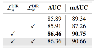
Both are required:
- One pushes anomalies towards their direction.
- The other keeps normal features near the origin.
Aggregated Output Losses
Removing any reduces performance, especially ![]() (forces even top-K to include some normality → improves robustness).
(forces even top-K to include some normality → improves robustness).
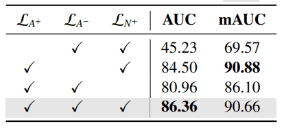
Regularizers
- Sparsity loss: encourages few frames to be anomalous.
- Smoothness loss: enforces temporal consistency.
- Both improve the realism and stability of predictions.
4.7 CLIP vs I3D Features
- Using I3D features (common in older anomaly detection works) instead of CLIP:
- Worse anomaly recognition.
- I3D embeddings don’t align with language → no semantic structure.
- CLIP embeddings + prompt learning → anomaly classes are more separable and interpretable.
5. Key Takeaways
- Innovation: AnomalyCLIP is the first LLV-based method for Video Anomaly Recognition.
- Strengths:
- Normality re-centering makes anomaly magnitude/direction interpretable.
- Selector model + CoOp prompts widen anomaly–normal separation.
- Axial Transformer captures temporal cues efficiently.
- Performance: Outperforms SOTA on ShanghaiTech, UCF-Crime, and XD-Violence.
- Practicality: Works under weak supervision (video-level labels only).
- Implementation: With our custom pipeline, you can run inference on arbitrary raw videos, save frames, get anomaly scores, per-class probs, and robust video-level anomaly predictions.
6. Conclusion
AnomalyCLIP marks a milestone in bridging foundation vision-language models with weakly supervised anomaly recognition. By redefining CLIP latent space with a normality prototype, introducing semantic prompt-based directions, and leveraging temporal transformers, it achieves state-of-the-art results in detecting and recognizing anomalies in videos.
Our deep dive not only explains its concepts but also shows practical ways to implement and extend it – from .npy feature inference to raw video analysis with per-frame visualization and majority-vote classification.
In short, AnomalyCLIP marks a significant step toward scalable, weakly supervised, and semantically rich video anomaly recognition, paving the way for real-world, fine-grained, multimodal AI systems.


