Explore the dynamic world of ADAS (Advanced Driver Assistance Systems) and the innovative field of stereo vision. In this article, we’ll explore how ADAS stereo vision in cars is changing the game, offering a smart alternative to the usual LiDAR-based methods for depth perception. This comprehensive research article includes a step-by-step pipeline on how to set up and fine-tune a STereo TRansformer (STTR) that can predict the disparity map from two camera streams, just like human eyes.
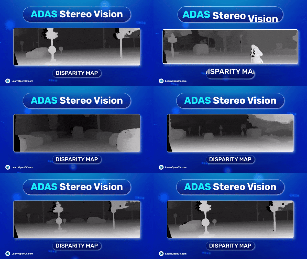
Instead of just pure computer vision theory, this article also includes real-world experimental results after fine-tuning the KITTI stereo vision dataset. The impressive results match what you’d expect from the more complex and expensive LiDAR systems. What’s more, you will also be able to explore the actual training and inference pipeline for such a model, which you won’t find in the basic guides. Get ready to learn about the latest car safety technology and how stereo vision is making a big impact!
To see the results, you may SCROLL BELOW to the concluding part of the article or click here to see the experimental results right away.
Why Stereo Vision?
ADAS stereo vision refers to the technique of using two cameras (akin to human eyes) to capture images from slightly different angles. This setup mimics human binocular vision, allowing the system to perceive the depth and 3D structure of the environment.
Key Technical Aspects of Stereo Vision
ADAS stereo vision has multiple advantages and highly complex functionalities. Let’s explore them to understand better:
- Epipolar Geometry and Depth Estimation: Stereo vision relies on epipolar geometry, a fundamental concept in computer vision that describes the geometric relationship between two views of a stereo setup. By finding corresponding points (features like edges or corners) in the pair of images, the system calculates the disparity (the difference in coordinates of similar features in both images). This disparity is inversely proportional to the camera’s scene depth, allowing for depth estimation.
- 3D Reconstruction and Point Cloud Generation: Through triangulation methods, stereo vision systems can reconstruct a 3D model of the observed scene. These systems generate a point cloud, where each point represents a physical location in the scene with 3D coordinates derived from the disparity map.
- Advantages Over LiDAR in Certain Aspects: It turns out that stereo vision is generally more cost-effective compared to 3D LiDAR systems. Cameras in stereo vision setups can capture high-resolution images, providing detailed texture information that is unavailable in LiDAR, at the moment. Furthermore, unlike LiDAR, which can struggle in certain lighting conditions (e.g., direct sunlight, dark environments), stereo vision systems can perform consistently across a wide range of lighting scenarios, especially with advancements in low-light imaging.
- Applications in ADAS: Cutting-edge capabilities such as Obstacle Detection and Avoidance, Lane Detection, Pedestrian Detection, etc are some valuable functions that stereo vision can contribute to.
The Idea of Disparity
In their research on enhancing ADAS stereo vision in computer vision applications, the authors Masatoshi Okutomi and Takeo Kanade [1] of ‘A Multiple-Baseline Stereo’ propose an innovative stereo matching method employing multiple stereo pairs with varied baselines to enhance distance estimation precision while mitigating ambiguity risks. The mathematical expression for disparity ![]() in stereo vision, which relates to the distance
in stereo vision, which relates to the distance ![]() from the camera, can be expressed using the baseline
from the camera, can be expressed using the baseline ![]() and the focal length
and the focal length ![]() of the camera. The expression is:
of the camera. The expression is:
![]()
In this formula, ![]() represents the disparity,
represents the disparity, ![]() is the baseline (the distance between the two camera centers),
is the baseline (the distance between the two camera centers), ![]() is the focal length of the camera, and
is the focal length of the camera, and ![]() is the distance to the object from the camera. The formula indicates that disparity is directly proportional to the product of the baseline and the focal length and inversely proportional to the distance to the object. This method circumvents the traditional trade-off between precision and accuracy in stereo matching by utilizing a lateral displacement of a camera to generate multiple images with different baselines.
is the distance to the object from the camera. The formula indicates that disparity is directly proportional to the product of the baseline and the focal length and inversely proportional to the distance to the object. This method circumvents the traditional trade-off between precision and accuracy in stereo matching by utilizing a lateral displacement of a camera to generate multiple images with different baselines.
The technique focuses on reducing global mismatches by calculating and summing the sum of squared-difference (SSD) values across these stereo pairs, represented against inverse distance rather than disparity. This approach effectively addresses inherent ambiguities in matching, such as repetitive scene patterns, and improves precision without resorting to search or sequential filtering techniques.

Literature Review – A look at Current Research Trends
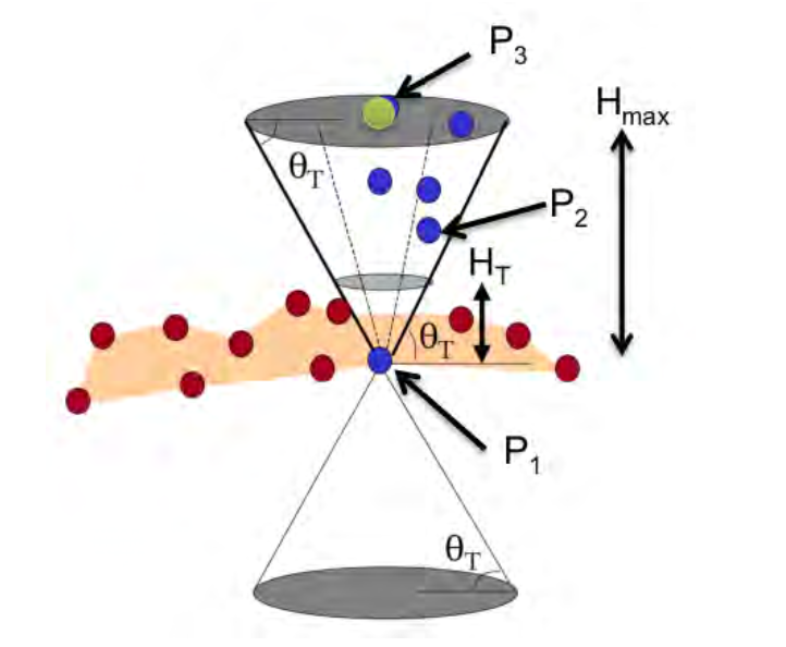
In their research paper, Naveen Appiah and Nitin Bandaru [2] introduced a novel methodology using dual 360° cameras for ADAS stereo, exploiting vertical camera displacement for comprehensive depth perception in all viewing directions. This approach primarily focuses on a geometry-based clustering technique for obstacle identification, where obstacles are defined as points or areas elevated from a ground plane. The obstacle detection algorithm quantitatively defines obstacles through two criteria: a vertical elevation difference between points ![]() constrained between minimum
constrained between minimum ![]() and maximum
and maximum ![]() heights and an angular threshold
heights and an angular threshold ![]() relative to a vertically displaced point
relative to a vertically displaced point ![]() . This method effectively employs a conical frustum in 3D space, determined by
. This method effectively employs a conical frustum in 3D space, determined by ![]() to classify points within as obstacles, enhancing the precision of environmental perception and aiding in motion planning for autonomous navigation.
to classify points within as obstacles, enhancing the precision of environmental perception and aiding in motion planning for autonomous navigation.
The research carried out by Hendrik Königshof [3] introduced a groundbreaking 3D object detection and pose estimation method tailored for automated driving. This method uniquely combines semantic data from a deep convolutional neural network (CNN) with disparity and geometric constraints, enabling the precise generation of 3D bounding boxes for various road users in real time.

The system employs a ResNet-38 based encoder for pixel-wise semantic segmentation and object detection, alongside a proposal-free bounding box detection mechanism influenced by SSD and RetinaNet. For disparity estimation on stereo video, it utilizes a GPU-accelerated block matching algorithm, leveraging a slanted planes approach and a novel confidence metric, CPKR, for reliable disparity determination. Integrating these techniques results in an efficient, real-time capable algorithm that demonstrates competitive performance on the KITTI 3D object detection benchmark, significantly outpacing existing image-based approaches in terms of runtime.
The paper ‘Revisiting Stereo Depth Estimation From a Sequence-to-Sequence Perspective with Transformers’, by Zhaoshuo Li et al., [4] introduced the Stereo Transformer (STTR) approach, a novel sequence-to-sequence methodology for stereo depth estimation. Unlike traditional methods, STTR employs dense pixel matching using positional information and attention mechanisms, bypassing the constraints of fixed disparity range and enhancing occlusion detection and confidence estimation.
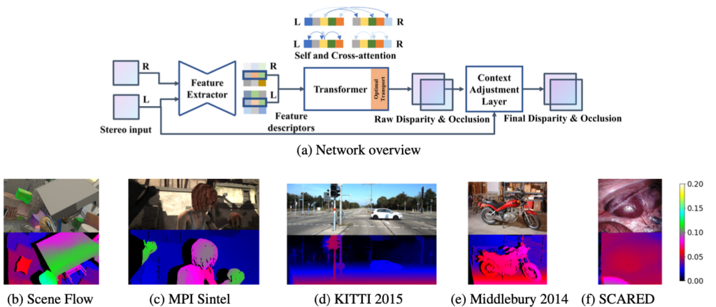
The architecture features an hourglass-shaped feature extractor with residual connections and spatial pyramid pooling for effective context acquisition. The Transformer model employs alternating self- and cross-attention layers, optimizing the feature descriptors for accurate disparity estimation. Unique to this model is the incorporation of entropy-regularized optimal transport for enforcing the uniqueness constraint in stereo matching, providing soft assignments with gradient flow. Additionally, STTR includes a context adjustment layer using convolution blocks and residual networks to refine the raw disparity and occlusion maps, leveraging cross-epipolar line information for enhanced accuracy in depth perception.
Overview of KITTI ADAS Stereo Vision Dataset
The KITTI 2015 ADAS Stereo Vision dataset [5,6], known for its application in computer vision and autonomous driving research, is a comprehensive and widely-used dataset. It was created as part of the KITTI Vision Benchmark Suite, a project by the Karlsruhe Institute of Technology and the Toyota Technological Institute at Chicago. The dataset consists of 200 training scenes and 200 test scenes. Each scene includes four color images, all saved in lossless PNG format. This structure provides a substantial amount of data for training and validation purposes.
A significant aspect of the KITTI 2015 dataset is its focus on dynamic scenes, which departs from earlier versions like the KITTI 2012. This inclusion of moving objects in the scenes makes it particularly relevant for applications in autonomous driving and other areas where understanding dynamic environments is crucial.
Before moving forward, let’s have a look at a few samples from this dataset, shall we?
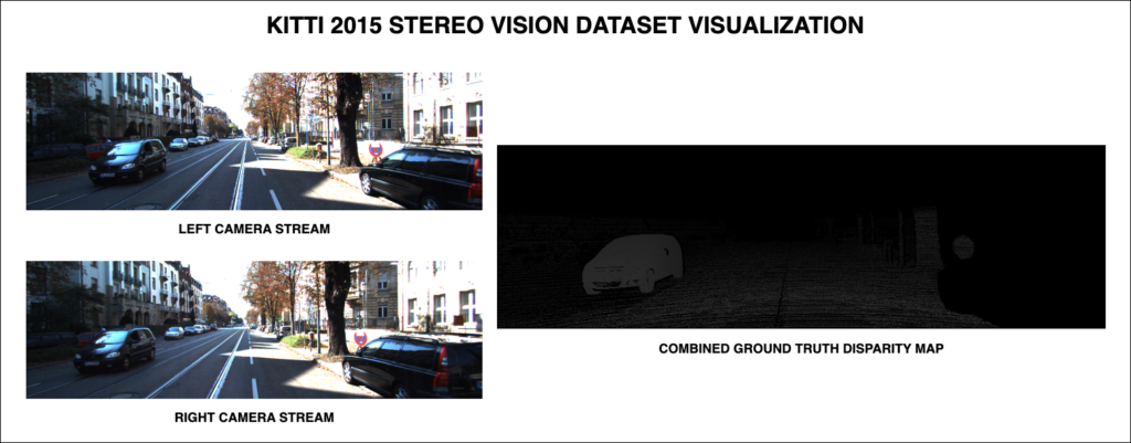
From the above FIGURE 5, we can observe that for each instance in unit time, there are three data-points:
- Left Camera Stream
- Right Camera Stream
- Combined Ground Truth Disparity Map
STereo TRansformer (STTR) – Architecture
In this comprehensive section, let’s explore the internal architecture of the STereo TRansformer (STTR) network. A detailed illustration of this model has also been shown below in FIGURE 6:

Highlights
- Feature Extractor: Employs an advanced hourglass architecture with residual connections and spatial pyramid pooling for comprehensive local and global context capture.
- Transformer: Utilizes an alternating self- and cross-attention mechanism, updating feature descriptors based on image context and positional relationships.
- Optimal Transport: Applies entropy-regularized optimal transport for soft assignment in stereo matching, ensuring flexibility and differentiability.
- Context Adjustment Layer: Refines disparity and occlusion estimations using convolution blocks and activations, integrating cross-epipolar line context.
- Memory-Feasible Implementation: Implements gradient checkpointing and mixed-precision training to manage memory efficiently, enabling scalability of the attention layers on standard hardware.
Feature Extractor
The Feature Extractor in STTR uses an hourglass-shaped architecture akin to prior models but with notable enhancements. It incorporates residual connections and spatial pyramid pooling modules for efficient global context acquisition. The decoding path is designed with transposed convolution, dense blocks, and a final convolution layer, ensuring that the feature descriptors for each pixel encode both local and global context and maintain the same spatial resolution as the input image.
class SppBackbone(nn.Module):
    """
    Contracting path of feature descriptor using Spatial Pyramid Pooling,
    SPP followed by PSMNet (https://github.com/JiaRenChang/PSMNet)
    """

    def __init__(self):
        super(SppBackbone, self).__init__()
        self.inplanes = 32
        self.in_conv = nn.Sequential(nn.Conv2d(3, 16, kernel_size=3, padding=1, stride=2, bias=False),
                                     nn.BatchNorm2d(16),
                                     nn.ReLU(inplace=True),
                                     nn.Conv2d(16, 16, kernel_size=3, padding=1, bias=False),
                                     nn.BatchNorm2d(16),
                                     nn.ReLU(inplace=True),
                                     nn.Conv2d(16, 32, kernel_size=3, padding=1, bias=False),
                                     nn.BatchNorm2d(32),
                                     nn.ReLU(inplace=True))  # 1/2

        self.resblock_1 = self._make_layer(BasicBlock, 64, 3, 2)  # 1/4
        self.resblock_2 = self._make_layer(BasicBlock, 128, 3, 2)  # 1/8

        self.branch1 = nn.Sequential(nn.AvgPool2d((16, 16), stride=(16, 16)),
                                     nn.Conv2d(128, 32, kernel_size=1, bias=False),
                                     nn.BatchNorm2d(32),
                                     nn.ReLU(inplace=True))

        self.branch2 = nn.Sequential(nn.AvgPool2d((8, 8), stride=(8, 8)),
                                     nn.Conv2d(128, 32, kernel_size=1, bias=False),
                                     nn.BatchNorm2d(32),
                                     nn.ReLU(inplace=True))

        self.branch3 = nn.Sequential(nn.AvgPool2d((4, 4), stride=(4, 4)),
                                     nn.Conv2d(128, 32, kernel_size=1, bias=False),
                                     nn.BatchNorm2d(32),
                                     nn.ReLU(inplace=True))

        self.branch4 = nn.Sequential(nn.AvgPool2d((2, 2), stride=(2, 2)),
                                     nn.Conv2d(128, 32, kernel_size=1, bias=False),
                                     nn.BatchNorm2d(32),
                                     nn.ReLU(inplace=True))

    def _make_layer(self, block, planes, blocks, stride=1):
        downsample = None
        if stride != 1 or self.inplanes != planes * block.expansion:
            downsample = nn.Sequential(nn.Conv2d(self.inplanes, planes * block.expansion,
                                                 kernel_size=1, stride=stride, bias=False),
                                       nn.BatchNorm2d(planes * block.expansion), )
        layers = []
        layers.append(block(self.inplanes, planes, stride, downsample))
        self.inplanes = planes * block.expansion
        for i in range(1, blocks):
            layers.append(block(self.inplanes, planes))
        return nn.Sequential(*layers)

    def forward(self, x: NestedTensor):
        """
        :param x: NestedTensor
        :return: list containing feature descriptors at different spatial resolution
                0: [2N, 3, H, W]
                1: [2N, C0, H//4, W//4]
                2: [2N, C1, H//8, W//8]
                3: [2N, C2, H//16, W//16]
        """
        _, _, h, w = x.left.shape

        src_stereo = torch.cat([x.left, x.right], dim=0)  # 2NxCxHxW

        # in conv
        output = self.in_conv(src_stereo)  # 1/2

        # res blocks
        output_1 = self.resblock_1(output)  # 1/4
        output_2 = self.resblock_2(output_1)  # 1/8

        # spp
        h_spp, w_spp = math.ceil(h / 16), math.ceil(w / 16)
        spp_1 = self.branch1(output_2)
        spp_1 = F.interpolate(spp_1, size=(h_spp, w_spp), mode='bilinear', align_corners=False)
        spp_2 = self.branch2(output_2)
        spp_2 = F.interpolate(spp_2, size=(h_spp, w_spp), mode='bilinear', align_corners=False)
        spp_3 = self.branch3(output_2)
        spp_3 = F.interpolate(spp_3, size=(h_spp, w_spp), mode='bilinear', align_corners=False)
        spp_4 = self.branch4(output_2)
        spp_4 = F.interpolate(spp_4, size=(h_spp, w_spp), mode='bilinear', align_corners=False)
        output_3 = torch.cat([spp_1, spp_2, spp_3, spp_4], dim=1)  # 1/16

        return [src_stereo, output_1, output_2, output_3]
Transformer
The Transformer architecture in STTR is a key component, employing an alternating attention mechanism. It utilizes self-attention for computing attention between pixels along the epipolar line in the same image and cross-attention for corresponding epipolar lines in left and right images. This approach alternates between self- and cross-attention for ![]() layers, continually updating the feature descriptors based on image context and relative position. The final layer of cross-attention focuses on estimating raw disparity, incorporating operations like optimal transport for compliance with uniqueness constraints and an attention mask for search space reduction.
layers, continually updating the feature descriptors based on image context and relative position. The final layer of cross-attention focuses on estimating raw disparity, incorporating operations like optimal transport for compliance with uniqueness constraints and an attention mask for search space reduction.
class Transformer(nn.Module):
    """
    Transformer computes self (intra image) and cross (inter image) attention
    """

    def __init__(self, hidden_dim: int = 128, nhead: int = 8, num_attn_layers: int = 6):
        super().__init__()

        self_attn_layer = TransformerSelfAttnLayer(hidden_dim, nhead)
        self.self_attn_layers = get_clones(self_attn_layer, num_attn_layers)

        cross_attn_layer = TransformerCrossAttnLayer(hidden_dim, nhead)
        self.cross_attn_layers = get_clones(cross_attn_layer, num_attn_layers)

        self.norm = nn.LayerNorm(hidden_dim)

        self.hidden_dim = hidden_dim
        self.nhead = nhead
        self.num_attn_layers = num_attn_layers

    def _alternating_attn(self, feat: torch.Tensor, pos_enc: torch.Tensor, pos_indexes: Tensor, hn: int):
        """
        Alternate self and cross attention with gradient checkpointing to save memory

        :param feat: image feature concatenated from left and right, [W,2HN,C]
        :param pos_enc: positional encoding, [W,HN,C]
        :param pos_indexes: indexes to slice positional encoding, [W,HN,C]
        :param hn: size of HN
        :return: attention weight [N,H,W,W]
        """

        global layer_idx
        # alternating
        for idx, (self_attn, cross_attn) in enumerate(zip(self.self_attn_layers, self.cross_attn_layers)):
            layer_idx = idx

            # checkpoint self attn
            def create_custom_self_attn(module):
                def custom_self_attn(*inputs):
                    return module(*inputs)

                return custom_self_attn

            feat = checkpoint(create_custom_self_attn(self_attn), feat, pos_enc, pos_indexes)

            # add a flag for last layer of cross attention
            if idx == self.num_attn_layers - 1:
                # checkpoint cross attn
                def create_custom_cross_attn(module):
                    def custom_cross_attn(*inputs):
                        return module(*inputs, True)

                    return custom_cross_attn
            else:
                # checkpoint cross attn
                def create_custom_cross_attn(module):
                    def custom_cross_attn(*inputs):
                        return module(*inputs, False)

                    return custom_cross_attn

            feat, attn_weight = checkpoint(create_custom_cross_attn(cross_attn), feat[:, :hn], feat[:, hn:], pos_enc,
                                           pos_indexes)

        layer_idx = 0
        return attn_weight

    def forward(self, feat_left: torch.Tensor, feat_right: torch.Tensor, pos_enc: Optional[Tensor] = None):
        """
        :param feat_left: feature descriptor of left image, [N,C,H,W]
        :param feat_right: feature descriptor of right image, [N,C,H,W]
        :param pos_enc: relative positional encoding, [N,C,H,2W-1]
        :return: cross attention values [N,H,W,W], dim=2 is left image, dim=3 is right image
        """

        # flatten NxCxHxW to WxHNxC
        bs, c, hn, w = feat_left.shape

        feat_left = feat_left.permute(1, 3, 2, 0).flatten(2).permute(1, 2, 0)  # CxWxHxN -> CxWxHN -> WxHNxC
        feat_right = feat_right.permute(1, 3, 2, 0).flatten(2).permute(1, 2, 0)
        if pos_enc is not None:
            with torch.no_grad():
                # indexes to shift rel pos encoding
                indexes_r = torch.linspace(w - 1, 0, w).view(w, 1).to(feat_left.device)
                indexes_c = torch.linspace(0, w - 1, w).view(1, w).to(feat_left.device)
                pos_indexes = (indexes_r + indexes_c).view(-1).long()  # WxW' -> WW'
        else:
            pos_indexes = None

        # concatenate left and right features
        feat = torch.cat([feat_left, feat_right], dim=1)  # Wx2HNxC

        # compute attention
        attn_weight = self._alternating_attn(feat, pos_enc, pos_indexes, hn)
        attn_weight = attn_weight.view(hn, bs, w, w).permute(1, 0, 2, 3)  # NxHxWxW, dim=2 left image, dim=3 right image

        return attn_weight
class TransformerSelfAttnLayer(nn.Module):
    """
    Self attention layer
    """

    def __init__(self, hidden_dim: int, nhead: int):
        super().__init__()
        self.self_attn = MultiheadAttentionRelative(hidden_dim, nhead)

        self.norm1 = nn.LayerNorm(hidden_dim)

    def forward(self, feat: Tensor,
                pos: Optional[Tensor] = None,
                pos_indexes: Optional[Tensor] = None):
        """
        :param feat: image feature [W,2HN,C]
        :param pos: pos encoding [2W-1,HN,C]
        :param pos_indexes: indexes to slice pos encoding [W,W]
        :return: updated image feature
        """
        feat2 = self.norm1(feat)

        # torch.save(feat2, 'feat_self_attn_input_' + str(layer_idx) + '.dat')

        feat2, attn_weight, _ = self.self_attn(query=feat2, key=feat2, value=feat2, pos_enc=pos,
                                               pos_indexes=pos_indexes)

        # torch.save(attn_weight, 'self_attn_' + str(layer_idx) + '.dat')

        feat = feat + feat2

        return feat
class TransformerCrossAttnLayer(nn.Module):
    """
    Cross attention layer
    """

    def __init__(self, hidden_dim: int, nhead: int):
        super().__init__()
        self.cross_attn = MultiheadAttentionRelative(hidden_dim, nhead)

        self.norm1 = nn.LayerNorm(hidden_dim)
        self.norm2 = nn.LayerNorm(hidden_dim)

    def forward(self, feat_left: Tensor, feat_right: Tensor,
                pos: Optional[Tensor] = None,
                pos_indexes: Optional[Tensor] = None,
                last_layer: Optional[bool] = False):
        """
        :param feat_left: left image feature, [W,HN,C]
        :param feat_right: right image feature, [W,HN,C]
        :param pos: pos encoding, [2W-1,HN,C]
        :param pos_indexes: indexes to slicer pos encoding [W,W]
        :param last_layer: Boolean indicating if the current layer is the last layer
        :return: update image feature and attention weight
        """
        feat_left_2 = self.norm1(feat_left)
        feat_right_2 = self.norm1(feat_right)

        # torch.save(torch.cat([feat_left_2, feat_right_2], dim=1), 'feat_cross_attn_input_' + str(layer_idx) + '.dat')

        # update right features
        if pos is not None:
            pos_flipped = torch.flip(pos, [0])
        else:
            pos_flipped = pos
        feat_right_2 = self.cross_attn(query=feat_right_2, key=feat_left_2, value=feat_left_2, pos_enc=pos_flipped,
                                       pos_indexes=pos_indexes)[0]

        feat_right = feat_right + feat_right_2

        # update left features
        # use attn mask for last layer
        if last_layer:
            w = feat_left_2.size(0)
            attn_mask = self._generate_square_subsequent_mask(w).to(feat_left.device)  # generate attn mask
        else:
            attn_mask = None

        # normalize again the updated right features
        feat_right_2 = self.norm2(feat_right)
        feat_left_2, attn_weight, raw_attn = self.cross_attn(query=feat_left_2, key=feat_right_2, value=feat_right_2,
                                                             attn_mask=attn_mask, pos_enc=pos,
                                                             pos_indexes=pos_indexes)

        # torch.save(attn_weight, 'cross_attn_' + str(layer_idx) + '.dat')

        feat_left = feat_left + feat_left_2

        # concat features
        feat = torch.cat([feat_left, feat_right], dim=1)  # Wx2HNxC

        return feat, raw_attn

    @torch.no_grad()
    def _generate_square_subsequent_mask(self, sz: int):
        """
        Generate a mask which is upper triangular

        :param sz: square matrix size
        :return: diagonal binary mask [sz,sz]
        """
        mask = torch.triu(torch.ones(sz, sz), diagonal=1)
        mask[mask == 1] = float('-inf')
        return mask
def build_transformer(args):
    return Transformer(
        hidden_dim=args.channel_dim,
        nhead=args.nheads,
        num_attn_layers=args.num_attn_layers
    )
In STTR, the attention modules use dot-product similarity to compute attention between query sets and key vectors, which are then used to weigh value vectors. The model adopts multi-head attention, enhancing the expressivity of the feature descriptor by dividing the channel dimension into groups, thereby optimizing attention calculations and improving feature representation.
Optimal Transport
The optimal transport component in STTR addresses the uniqueness constraint in stereo matching. Unlike hard assignments in previous models that hindered gradient flow, the STTR uses entropy-regularized optimal transport for its soft assignment properties and differentiability. This approach is beneficial for tasks like sparse feature and semantic correspondence matching, providing a more flexible and efficient matching process.
Context Adjustment Layer
This layer addresses the lack of cross-epipolar line context in raw disparity and occlusion maps. By concatenating these maps with the left image and using convolution blocks and ReLU activation, the model refines the disparity estimates. Using sigmoid activation for final occlusion estimation and incorporating residual blocks for disparity refinement ensures a comprehensive adjustment based on the input image context.
class ContextAdjustmentLayer(nn.Module):
    """
    Adjust the disp and occ based on image context, design loosely follows https://github.com/JiahuiYu/wdsr_ntire2018
    """

    def __init__(self, num_blocks=8, feature_dim=16, expansion=3):
        super().__init__()
        self.num_blocks = num_blocks

        # disp head
        self.in_conv = nn.Conv2d(4, feature_dim, kernel_size=3, padding=1)
        self.layers = nn.ModuleList([ResBlock(feature_dim, expansion) for _ in range(num_blocks)])
        self.out_conv = nn.Conv2d(feature_dim, 1, kernel_size=3, padding=1)

        # occ head
        self.occ_head = nn.Sequential(
            weight_norm(nn.Conv2d(1 + 3, feature_dim, kernel_size=3, padding=1)),
            weight_norm(nn.Conv2d(feature_dim, feature_dim, kernel_size=3, padding=1)),
            nn.ReLU(inplace=True),
            weight_norm(nn.Conv2d(feature_dim, feature_dim, kernel_size=3, padding=1)),
            weight_norm(nn.Conv2d(feature_dim, feature_dim, kernel_size=3, padding=1)),
            nn.ReLU(inplace=True),
            nn.Conv2d(feature_dim, 1, kernel_size=3, padding=1),
            nn.Sigmoid()
        )

    def forward(self, disp_raw: Tensor, occ_raw: Tensor, img: Tensor):
        """
        :param disp_raw: raw disparity, [N,1,H,W]
        :param occ_raw: raw occlusion mask, [N,1,H,W]
        :param img: input left image, [N,3,H,W]
        :return:
            disp_final: final disparity [N,1,H,W]
            occ_final: final occlusion [N,1,H,W]
        """""
        feat = self.in_conv(torch.cat([disp_raw, img], dim=1))
        for layer in self.layers:
            feat = layer(feat, disp_raw)
        disp_res = self.out_conv(feat)
        disp_final = disp_raw + disp_res

        occ_final = self.occ_head(torch.cat([occ_raw, img], dim=1))

        return disp_final, occ_final
Memory-Feasible Implementation
STTR addresses the high memory consumption typically associated with attention mechanisms. It utilizes techniques like gradient checkpointing, mixed-precision training, and attention stride adjustment to manage memory usage effectively. These approaches reduce the memory footprint and allow the network to scale in terms of the number of attention layers, making it practical for use on conventional hardware.
Code Walkthrough – STTR
Fine-Tuning Strategy
As mentioned previously in this article, the dataset of choice for this fine-tuning procedure is KITTI ADAS stereo vision 2015. However, the 2012 version of the same dataset is also still available as an open-source download. Preprocessing the raw dataset is crucial in any deep learning pipeline. It is important to understand that the below preprocessing script supports both 2015 and 2012 versions of the dataset, or it can be used in conjunction with each other also.
class KITTIBaseDataset(data.Dataset):
    def __init__(self, datadir, split='train'):
        super(KITTIBaseDataset, self).__init__()

        self.datadir = datadir
        self.split = split

        if split == 'train' or split == 'validation' or split == 'validation_all':
            self.sub_folder = 'training/'
        elif split == 'test':
            self.sub_folder = 'testing/'

        # to be set by child classes
        self.left_fold = None
        self.right_fold = None
        self.disp_fold = None

        self._augmentation()

    def _read_data(self):
        assert self.left_fold is not None

        self.left_data = natsorted([os.path.join(self.datadir, self.sub_folder, self.left_fold, img) for img in
                                    os.listdir(os.path.join(self.datadir, self.sub_folder, self.left_fold)) if
                                    img.find('_10') > -1])
        self.right_data = [img.replace(self.left_fold, self.right_fold) for img in self.left_data]
        self.disp_data = [img.replace(self.left_fold, self.disp_fold) for img in self.left_data]

        self._split_data()

    def _split_data(self):
        train_val_frac = 0.95
        # split data
        if len(self.left_data) > 1:
            if self.split == 'train':
                self.left_data = self.left_data[:int(len(self.left_data) * train_val_frac)]
                self.right_data = self.right_data[:int(len(self.right_data) * train_val_frac)]
                self.disp_data = self.disp_data[:int(len(self.disp_data) * train_val_frac)]
            elif self.split == 'validation':
                self.left_data = self.left_data[int(len(self.left_data) * train_val_frac):]
                self.right_data = self.right_data[int(len(self.right_data) * train_val_frac):]
                self.disp_data = self.disp_data[int(len(self.disp_data) * train_val_frac):]

    def _augmentation(self):
        if self.split == 'train':
            self.transformation = Compose([
                RGBShiftStereo(always_apply=True, p_asym=0.5),
                RandomBrightnessContrastStereo(always_apply=True, p_asym=0.5)
            ])
        elif self.split == 'validation' or self.split == 'test' or self.split == 'validation_all':
            self.transformation = None
        else:
            raise Exception("Split not recognized")

    def __len__(self):
        return len(self.left_data)

    def __getitem__(self, idx):
        input_data = {}

        # left
        left_fname = self.left_data[idx]
        left = np.array(Image.open(left_fname)).astype(np.uint8)
        input_data['left'] = left

        # right
        right_fname = self.right_data[idx]
        right = np.array(Image.open(right_fname)).astype(np.uint8)
        input_data['right'] = right

        # disp
        if not self.split == 'test':  # no disp for test files
            disp_fname = self.disp_data[idx]

            disp = np.array(Image.open(disp_fname)).astype(float) / 256.
            input_data['disp'] = disp
            input_data['occ_mask'] = np.zeros_like(disp).astype(bool)

            if self.split == 'train':
                input_data = random_crop(200, 640, input_data, self.split)

            input_data = augment(input_data, self.transformation)
        else:
            input_data = normalization(**input_data)

        return input_data
class KITTIDataset(KITTIBaseDataset):
    """
    Merged KITTI dataset with 2015 and 2012 data
    """

    def __init__(self, datadir, split='train'):
        super(KITTIDataset, self).__init__(datadir, split)

        self.left_fold_2015 = 'image_2'
        self.right_fold_2015 = 'image_3'
        self.disp_fold_2015 = 'disp_occ_0'  # we read disp data with occlusion since we compute occ directly
        self.preprend_2015 = '2015'

        self.left_fold_2012 = 'colored_0'
        self.right_fold_2012 = 'colored_1'
        self.disp_fold_2012 = 'disp_occ'  # we we read disp data with occlusion since we compute occ directly
        self.preprend_2012 = '2012'

        self._read_data()

    def _read_data(self):
        assert self.left_fold_2015 is not None
        assert self.left_fold_2012 is not None

        left_data_2015 = [os.path.join(self.datadir, self.preprend_2015, self.sub_folder, self.left_fold_2015, img) for
                          img in os.listdir(os.path.join(self.datadir, '2015', self.sub_folder, self.left_fold_2015)) if
                          img.find('_10') > -1]
        left_data_2015 = natsorted(left_data_2015)
        right_data_2015 = [img.replace(self.left_fold_2015, self.right_fold_2015) for img in left_data_2015]
        disp_data_2015 = [img.replace(self.left_fold_2015, self.disp_fold_2015) for img in left_data_2015]

        left_data_2012 = [os.path.join(self.datadir, self.preprend_2012, self.sub_folder, self.left_fold_2012, img) for
                          img in os.listdir(os.path.join(self.datadir, '2012', self.sub_folder, self.left_fold_2012)) if
                          img.find('_10') > -1]
        left_data_2012 = natsorted(left_data_2012)
        right_data_2012 = [img.replace(self.left_fold_2012, self.right_fold_2012) for img in left_data_2012]
        disp_data_2012 = [img.replace(self.left_fold_2012, self.disp_fold_2012) for img in left_data_2012]

        self.left_data = natsorted(left_data_2015 + left_data_2012)
        self.right_data = natsorted(right_data_2015 + right_data_2012)
        self.disp_data = natsorted(disp_data_2015 + disp_data_2012)

        self._split_data()
class KITTI2015Dataset(KITTIBaseDataset):
    def __init__(self, datadir, split='train'):
        super(KITTI2015Dataset, self).__init__(datadir, split)

        self.left_fold = 'image_2/'
        self.right_fold = 'image_3/'
        self.disp_fold = 'disp_occ_0/'  # we read disp data with occlusion since we compute occ directly

        self._read_data()


class KITTI2012Dataset(KITTIBaseDataset):
    def __init__(self, datadir, split='train'):
        super(KITTI2012Dataset, self).__init__(datadir, split)

        self.left_fold = 'colored_0/'
        self.right_fold = 'colored_1/'
        self.disp_fold = 'disp_occ/'  # we read disp data with occlusion since we compute occ directly

        self._read_data()
Let’s try to understand this snippet in detail:
- KITTIBaseDataset: This is a base class for handling KITTI datasets. It is inherited from
torch.utils.data.Dataset. The constructor (__init__) takes two parameters:datadir(directory containing the dataset) andsplit(specifying the data split – train, validation, test, etc.). It initializes dataset paths and calls the_augmentation()method to set up data augmentation strategies based on the data split. The_read_data()method constructs paths for left, right, and disparity images and splits the dataset into training and validation sets. The_split_data()method splits the data into training and validation sets based on a predetermined fraction, and the_augmentation()method defines data augmentation strategies for training data, such as RGB shifts and random brightness / contrast adjustments. - KITTI2015Dataset and KITTI2012Dataset: These classes inherit from
KITTIBaseDataset. They specialize in handling the KITTI 2015 and KITTI 2012 datasets, respectively. Each class sets the specific directories (left_fold,right_fold,disp_fold) for the left, right, and disparity images according to the dataset structure. - KITTIDataset: This class also inherits from
KITTIBaseDataset. It is designed to handle a merged dataset comprising of KITTI 2015 and KITTI 2012 data. It sets separate directory paths for each year’s data and then reads and merges them, and the_read_data()method is overridden to accommodate the reading and merging of data from both datasets.
For the above script to work, a specific dataset hierarchy needs to be set up. If you download the code using the code package provided in this research article, the structure will already have been applied. However, if you wish to download the raw KITTI ADAS stereo vision dataset on your own, here is the link:
Let’s explore the directory structure as well:
stereo-transformer
├── sample_data
│   └── KITTI_2015
│   		├── 2012
│		│	├──  testing
│		│	│	├── colored_0
│		│	│	├── colored_1
│		│	│	├── image_0
│		│	│	└── training
│		│	└── training
│		│		├── colored_0
│		│		├── colored_1
│		│		└── disp_occ
│		└── 2015
│			├── testing
│			│	├── image_2
│			│	└── disp_occ
│			└── training
│				├── image_2
│				├── image_3
│				└── disp_occ_0
├── dataset
├── media
├── module
├── run
├── scripts
└── utilities
To start the fine-tuning process, you can just fire up the below command from within the root directory of the stereo-transformer.
python main.py  --epochs 400\
                --batch_size 1\
                --checkpoint kitti_ft\
                --num_workers 2\
                --dataset kitti\
                --dataset_directory sample_data/KITTI_2015\
                --ft\
                --resume kitti_finetuned_model.pth.tar
This command takes few arguments as inputs:
- No. of Epochs
- Batch Size
- Checkpoint Directory
- No. of Workers
- Dataset Type
- Dataset Directory
- Resume Checkpoint Directory
Depending on your compute resources, you may increase the number of Epochs, Batch Size, and Workers.
NOTE: Initially, this fine-tuning experiment was tested on a deep learning machine with an Nvidia RTX 3080 Ti. But, it quickly ran out of vRAM. Hence, an Nvidia RTX A5000 w/ 24GB vRAM was used to fine-tune this STTR model for ADAS stereo vision.
def print_param(model):
    """
    print number of parameters in the model
    """

    n_parameters = sum(p.numel() for n, p in model.named_parameters() if 'backbone' in n and p.requires_grad)
    print('number of params in backbone:', f'{n_parameters:,}')
    n_parameters = sum(p.numel() for n, p in model.named_parameters() if
                       'transformer' in n and 'regression' not in n and p.requires_grad)
    print('number of params in transformer:', f'{n_parameters:,}')
    n_parameters = sum(p.numel() for n, p in model.named_parameters() if 'tokenizer' in n and p.requires_grad)

    print('number of params in tokenizer:', f'{n_parameters:,}')
    n_parameters = sum(p.numel() for n, p in model.named_parameters() if 'regression' in n and p.requires_grad)
    print('number of params in regression:', f'{n_parameters:,}')
def main(args):
    # get device
    device = torch.device(args.device)

    # fix the seed for reproducibility
    seed = args.seed
    torch.manual_seed(seed)
    np.random.seed(seed)
    random.seed(seed)

    # build model
    model = STTR(args).to(device)
    print_param(model)

    # set learning rate
    param_dicts = [
        {"params": [p for n, p in model.named_parameters() if
                    "backbone" not in n and "regression" not in n and p.requires_grad]},
        {
            "params": [p for n, p in model.named_parameters() if "backbone" in n and p.requires_grad],
            "lr": args.lr_backbone,
        },
        {
            "params": [p for n, p in model.named_parameters() if "regression" in n and p.requires_grad],
            "lr": args.lr_regression,
        },
    ]

    # define optimizer and learning rate scheduler
    optimizer = torch.optim.AdamW(param_dicts, lr=args.lr, weight_decay=args.weight_decay)
    lr_scheduler = torch.optim.lr_scheduler.ExponentialLR(optimizer, gamma=args.lr_decay_rate)

    # mixed precision training
    if args.apex:
        from apex import amp
        model, optimizer = amp.initialize(model, optimizer, opt_level='O1')
    else:
        amp = None

    # load checkpoint if provided
    prev_best = np.inf
    if args.resume != '':
        if not os.path.isfile(args.resume):
            raise RuntimeError(f"=> no checkpoint found at '{args.resume}'")
        checkpoint = torch.load(args.resume)

        pretrained_dict = checkpoint['state_dict']
        missing, unexpected = model.load_state_dict(pretrained_dict, strict=False)
        # check missing and unexpected keys
        if len(missing) > 0:
            print("Missing keys: ", ','.join(missing))
            raise Exception("Missing keys.")
        unexpected_filtered = [k for k in unexpected if
                               'running_mean' not in k and 'running_var' not in k]  # skip bn params
        if len(unexpected_filtered) > 0:
            print("Unexpected keys: ", ','.join(unexpected_filtered))
            raise Exception("Unexpected keys.")
        print("Pre-trained model successfully loaded.")

        # if not ft/inference/eval, load states for optimizer, lr_scheduler, amp and prev best
        if not (args.ft or args.inference or args.eval):
            if len(unexpected) > 0:  # loaded checkpoint has bn parameters, legacy resume, skip loading
                raise Exception("Resuming legacy model with BN parameters. Not possible due to BN param change. " +
                                "Do you want to finetune or inference? If so, check your arguments.")
            else:
                args.start_epoch = checkpoint['epoch'] + 1
                optimizer.load_state_dict(checkpoint['optimizer'])
                lr_scheduler.load_state_dict(checkpoint['lr_scheduler'])
                prev_best = checkpoint['best_pred']
                if args.apex:
                    amp.load_state_dict(checkpoint['amp'])
                print("Pre-trained optimizer, lr scheduler and stats successfully loaded.")

    # inference
    if args.inference:
        print("Start inference")
        _, _, data_loader = build_data_loader(args)
        inference(model, data_loader, device, args.downsample)

        return

    # initiate saver and logger
    checkpoint_saver = Saver(args)
    summary_writer = TensorboardSummary(checkpoint_saver.experiment_dir)

    # build dataloader
    data_loader_train, data_loader_val, _ = build_data_loader(args)

    # build loss criterion
    criterion = build_criterion(args)

    # set downsample rate
    set_downsample(args)

    # eval
    if args.eval:
        print("Start evaluation")
        evaluate(model, criterion, data_loader_val, device, 0, summary_writer, True)
        return

    # train
    print("Start training")
    for epoch in range(args.start_epoch, args.epochs):
        # train
        print("Epoch: %d" % epoch)
        train_one_epoch(model, data_loader_train, optimizer, criterion, device, epoch, summary_writer,
                        args.clip_max_norm, amp)

        # step lr if not pretraining
        if not args.pre_train:
            lr_scheduler.step()
            print("current learning rate", lr_scheduler.get_lr())

        # empty cache
        torch.cuda.empty_cache()

        # save if pretrain, save every 50 epochs
        if args.pre_train or epoch % 50 == 0:
            save_checkpoint(epoch, model, optimizer, lr_scheduler, prev_best, checkpoint_saver, False, amp)

        # validate
        eval_stats = evaluate(model, criterion, data_loader_val, device, epoch, summary_writer, False)
        # save if best
        if prev_best > eval_stats['epe'] and 0.5 > eval_stats['px_error_rate']:
            save_checkpoint(epoch, model, optimizer, lr_scheduler, prev_best, checkpoint_saver, True, amp)

    # save final model
    save_checkpoint(epoch, model, optimizer, lr_scheduler, prev_best, checkpoint_saver, False, amp)

    return
Let’s try to understand what happens internally when you execute the above command in your development environment:
print_paramFunction: This function calculates and prints the number of parameters in different parts of the STTR model such as the backbone, transformer, tokenizer, and regression components. It uses PyTorch’snamed_parametersmethod for this purpose.- The core function of the script is handled by the
main()function. It sets up the computing device (CPU/GPU) based on the provided arguments. Ensures reproducibility of results by fixing the seed for random number generators in PyTorch, NumPy, and therandomlibrary. Initializes the STTR model and transfers it to the specified computing device. Callsprint_paramto display the number of parameters in each component of the model. - Configures different learning rates for various parts of the model, e.g., backbone. Defines the optimizer (AdamW) and learning rate scheduler (ExponentialLR) for training the model. Optionally employs mixed precision training for enhanced performance, using Nvidia’s Apex library. If a checkpoint path is provided, it loads the model state along with the optimizer, scheduler, and AMP states from the checkpoint for resuming training or fine-tuning.
- The script loads the data and runs the model in inference mode to make predictions, builds data loaders for training and validation datasets, sets up the loss function (criterion) for the model.
- The
main()function also contains a loop for training the model over multiple epochs, including calls for training and validation functions. It also includes LR scheduler stepping and model checkpointing based on validation performance. After training, the final model state is saved as a checkpoint.
Inference Strategy
We now have a fine-tuned model. But, how to perform inference on this model to check how it stacks up? In this section, let’s explore the inference pipeline for the fine-tuned STTR model. From the directory, refer to the inference-kitti.ipynb file within the scripts sub-directory.
from PIL import Image
import torch
import numpy as np
import cv2
import glob
import os


import argparse
import matplotlib.pyplot as plt
import sys
sys.path.append('../') # add relative path

from module.sttr import STTR
from dataset.preprocess import normalization, compute_left_occ_region
from utilities.misc import NestedTensor
Initially, the necessary packages such as PIL, torch, cv2, glob, os and other internal dependencies must be imported.
# Function to load images
def load_images(image_dir, pattern):
    filenames = sorted(glob.glob(os.path.join(image_dir, pattern)))
    return [np.array(Image.open(filename)) for filename in filenames[:500]]
In this code snippet, about 500 image pairs from the KITTI ADAS stereo vision dataset’s test folder is used for inference.
# Default parameters
args = type('', (), {})() # create empty args
args.channel_dim = 128
args.position_encoding = 'sine1d_rel'
args.num_attn_layers = 6
args.nheads = 8
args.regression_head = 'ot'
args.context_adjustment_layer = 'cal'
args.cal_num_blocks = 8
args.cal_feat_dim = 16
args.cal_expansion_ratio = 4
Every model takes in a few parameters called args as input to create an instance of that specific model. In this case, the above arguments are the default parameters.
model = STTR(args).cuda().eval()
Since we are performing inference on the already fine-tuned model, the model has to be set to evaluation mode.
# Load the pretrained model
model_file_name = "../kitti_finetuned_model.pth.tar"
checkpoint = torch.load(model_file_name)
pretrained_dict = checkpoint['state_dict']
model.load_state_dict(pretrained_dict, strict=False) # prevent BN parameters from breaking the model loading
print("Pre-trained model successfully loaded.")
In the above code snippet, the pre-trained model has been loaded with its last saved checkpoint file.
# Load images
left_images = load_images('../sample_data/KITTI_2015/2015/training/image_2', '*.png')
right_images = load_images('../sample_data/KITTI_2015/2015/training/image_3', '*.png')
Directory paths to the left and right images from the testing set of the KITTI ADAS stereo vision dataset have been initialized.
# Initialize output directory and image dimensions
height, width, _ = left_images[0].shape
output_dir = '../inference_output/'
os.makedirs(output_dir, exist_ok=True)  # Create output directory if it doesn't exist
There needs to be a directory into which the inference results are stored, right? For this, a folder called inference_output will be created automatically by the script into which all the results will be stored.
for i, (left, right) in enumerate(zip(left_images, right_images)):
    # Normalize and create NestedTensor for each set of images
    input_data = normalization(left=left, right=right)
    h, w, _ = left.shape
    bs = 1
    downsample = 3
    col_offset = int(downsample / 2)
    row_offset = int(downsample / 2)
    sampled_cols = torch.arange(col_offset, w, downsample)[None,].expand(bs, -1).cuda()
    sampled_rows = torch.arange(row_offset, h, downsample)[None,].expand(bs, -1).cuda()
    input_data = NestedTensor(input_data['left'].cuda()[None,], input_data['right'].cuda()[None,], sampled_cols=sampled_cols, sampled_rows=sampled_rows)

    # Perform inference
    output = model(input_data)
    disp_pred = output['disp_pred'].data.cpu().numpy()[0]
    occ_pred = output['occ_pred'].data.cpu().numpy()[0] > 0.5
    disp_pred[occ_pred] = 0.0

     # Ensure disp_pred and occ_pred are normalized and converted to uint8
    disp_pred_norm = cv2.normalize(disp_pred, None, 0, 255, cv2.NORM_MINMAX).astype(np.uint8)
    occ_pred_uint8 = np.uint8(occ_pred * 255)

    # Combine predicted disparity and occlusion map
    combined_output = np.hstack((disp_pred_norm, occ_pred_uint8))

    # Save the combined output as a PNG file
    output_filename = os.path.join(output_dir, f'inference_{i:03d}.png')
    cv2.imwrite(output_filename, combined_output)
    print(f"Saved: {output_filename}")

print("All inferences saved as PNG files.")
The above code snippet processes a series of stereo image pairs (left and right images) for computer vision tasks using a deep learning model, focusing on disparity and occlusion predictions. It starts by iterating over pairs of left and right images. For each pair, the images are normalized and transformed into a custom data structure, likely a NestedTensor, which includes the images along with sampled column and row indices determined by a downsampling factor. This structure is then fed into a model for inference.
The model outputs predictions for disparity and occlusion, which are transferred from GPU to CPU memory and converted to NumPy arrays. The disparity predictions undergo normalization to the 8-bit format using OpenCV, and the occlusion predictions are thresholded to create a binary mask, which is also converted to an 8-bit format. The disparity predictions are adjusted by setting values to zero in occluded regions.
These processed predictions for disparity and occlusion are then combined into a single image and saved as a PNG file. The file names are generated using a loop counter to ensure uniqueness. The process repeats for each image pair, and upon completion, the script prints a message indicating that all inferences have been saved as PNG files. This pipeline effectively demonstrates a typical workflow for handling stereo image data in computer vision applications, from preprocessing to model inference and saving the results.
Experimental Results: Stereo Vision Disparity Map
In this section, let’s visualize the results from this research work:


Interesting results, right? SCROLL UP or have a look at the code walkthrough section of this research article to explore the intricate fine-tuning procedure.
Key Takeaways
In the previous section the inference outputs from the ADAS stereo vision transformer has been shown. Let’s analyze the key takeaways from this research work:
- Enhanced Depth Perception with STTR: Fine-tuning the Stereo Transformer (STTR) model significantly improves depth perception in ADAS, particularly excelling in challenging conditions such as low light and dynamic environments. This indicates the STTR model’s robustness and versatility in generating accurate disparity and occlusion maps.
- Stereo Vision as a Cost-Effective 3D LiDAR Alternative: Stereo vision offers detailed texture information and consistent performance across various lighting conditions, which LiDAR systems might lack.
- Computational and Performance Limitations: Despite its advantages, the STTR model poses significant computational demands, especially for real-time applications.
- Detection using Depth Estimation in ADAS: The research demonstrates the model’s potential capabilities in key ADAS functionalities such as obstacle detection and pedestrian detection. These applications benefit from the model’s ability to accurately detect and analyze environmental elements, aiding in safer and more efficient autonomous navigation.
Conclusions
In this research on ADAS stereo vision, we explored the use of Stereo Vision as an alternative to 3D LiDAR, focusing on fine-tuning the Stereo Transformer (STTR) model on KITTI ADAS stereo vision dataset. This resulted in significantly improved performance in depth perception, especially in low light and dynamic environments, suggesting that STTR is a viable, cost-effective alternative to LiDAR in ADAS. However, challenges remain in its computational demands and performance in extreme weather or low-texture environments.
References
[1] M. Okutomi and T. Kanade, “A multiple-baseline stereo,” in IEEE Transactions on Pattern Analysis and Machine Intelligence, vol. 15, no. 4, pp. 353-363, April 1993, doi: 10.1109/34.206955.
[2] Appiah, Naveen and Nitin Bandaru. “Obstacle detection using stereo vision for self-driving cars.” (2015).
[3] H. Königshof, N. O. Salscheider and C. Stiller, “Realtime 3D Object Detection for Automated Driving Using Stereo Vision and Semantic Information,” 2019 IEEE Intelligent Transportation Systems Conference (ITSC), Auckland, New Zealand, 2019, pp. 1405-1410, doi: 10.1109/ITSC.2019.8917330.
[4] Z. Li et al., “Revisiting Stereo Depth Estimation From a Sequence-to-Sequence Perspective with Transformers,” 2021 IEEE/CVF International Conference on Computer Vision (ICCV), Montreal, QC, Canada, 2021, pp. 6177-6186, doi: 10.1109/ICCV48922.2021.00614.
[5] Menze, Moritz, Christian Heipke, and Andreas Geiger. “Object Scene Flow.” ISPRS Journal of Photogrammetry and Remote Sensing (JPRS), 2018.
[6] Menze, Moritz, Christian Heipke, and Andreas Geiger. “Joint 3D Estimation of Vehicles and Scene Flow.” ISPRS Workshop on Image Sequence Analysis (ISA), 2015.

